Modeling & ComputationModelado y Computación
Learning Models: Supervised Learning.
Intro to Learning Models. Supervised Learning. Univariate Linear Regression.
0. Index.
-
Multiple Input Features.
-
Vectorization.
- 2.1. Mathematical concept.
- 2.2. Vectorization with python.
- 2.2.1. Python and C.
- 2.2.2. Numpy.
- 2.2.3. Numpy basic usage.
- 2.2.3.1. Importing Numpy.
- 2.2.3.2. Vectors and Numpy arrays.
- 2.2.3.3. Operation on vectors.
- 2.2.3.4. Matrix and operation with matrices.
-
Multiple Linear Regression.
- 3.1. Defining the problem.
- 3.2. Writing our code.
1. Learning Models.
1.1. Introduction. Problem setup.
In the first section we talked about a model to find an approximation of an unknown relation between two variable sets $\mathcal{X}$ and $\mathcal{Y}$.
This model consists of a template about this procedure based on an iterative process to find the local minimum of the function that measures the error of the hypothesis over the training set. Minimizing the error results in a "fair", reliable approximation of the sought relation.
This template's components are:
-
An input space $\mathcal{X}$ and output space $\mathcal{Y}$. This is where the relation lives and where the predictions want to be made.
-
The training set $\mathcal{D}$, this is what the model consumes to optimize the approximation.
-
A hypothesis set $\mathcal{H} = {h_\theta \mid \theta \in \Theta \subseteq \mathbb{R}^p}$. The family of functions which determines the model's expressiveness; what patterns it can and cannot represent.
-
A loss function $L : \mathcal{Y} \times \mathcal{Y} \to \mathbb{R}_{\geq 0}$. How do we measure error.
-
A cost function $J(\theta)$. How the loss function gets aggregated across the training data. This determines what is optimized and what gets parametrized by $\theta$ and decides the behavior of the model.
-
An optimization algorithm.
Every distinct decision over these parameters results in what we call a learning model. The learning models are in fact instantiations of the template we described in the post before. Most of the changes affect components $1$, $3$ and $4$; the cost function and the gradient descent remain the same over the models we will see in this blog.
1.2. Learning Model. Learning Paradigms.
Essentially, what we presented above is the problem setup, the parts of the problem we want to solve.
A problem setup is a tuple:
\[\mathcal{P} = (\mathcal{X}, \mathcal{Y}, \mathcal{D}, \mathcal{H}, L, J)\]With fixed data, this is, given $(\mathcal{X}, \mathcal{Y}, \mathcal{D})$, then we decide the learning model, this is, how the model predicts and how we calibrate how well it predicts (the hypothesis set and the loss function).
Thus, a learning model is a pair:
\[M:=(\mathcal{H}, L)\]This way, linear regression model means; learning model of affine transformation hypothesis and squared loss function: $M_{lr}:=(H_{at},L_s)$
2. Supervised Learning.
1.2.1.1. Definition.
Supervised Learning is one of the three best-known learning models, which trains a program to infer a relation between two data sets (inputs and outputs).
This training model relies on the fact that the program has a collection of pairs of inputs and outputs related by an unknown rule: $(x,y) \in \mathcal{X} \times \mathcal{Y} : y = f(x)$, and $f$ remains unknown (this function is typically an unknown joint distribution $P(X,Y)$, a stochastic relation; the function is a concrete case where all noise vanishes).
In this sense, supervised learning refers to the fact that during training (algorithm execution), every input $x$ comes with a label $y$; a correct answer that "supervises" the learning process.
In this sense, the task of supervised learning is, given the training set: ${ (x^{(i)}, y^{(i)}) }_{i=1}^{n} \subset \mathcal{X} \times \mathcal{Y}$ find some hypothesis $h : \mathcal{X} \to \mathcal{Y}$ of some hypothesis class $\mathcal{H}$ that minimizes the expected risk. However, taking again that $f$ is a simplification of $P$, in general, what is measured is the empirical risk instead which we call:
\[\hat{R}(h) = \frac{1}{n} \sum_{i=1}^{n} \ell\bigl(h(x^{(i)}), y^{(i)}\bigr)\]which basically measures the risk over the gathered sample instead of the entire population (which often is inaccessible in real problems).
Let's observe that this empirical risk is a template with three factors:
- The hypothesis class $h$ that makes the prediction against the labeled data.
- The loss function $\ell$ which measures the error between each pair $(h(x)^{(i)},y^{(i)})$
- A convenient scaling $\frac{1}{n}$; for convenience we can scale the empirical risk to simplify the result.
Later we will select each one of the three factors to instantiate the empirical risk into the cost function $J$.
1.2.1.2. Linear Regression: The simplest Supervised Learning Model instantiation.
Linear Regression is the simplest instantiation of the Supervised Learning Model.
Let's take a moment to introduce the affine concept. Linear and Affine are ways to apply transformations over the data on a set of points which satisfy specific conditions.
-
Linearity applies a scalar transformation over the data, in linear algebra we did learn that a linear transformation $f$ satisfies:
\[f(\alpha u + \beta v) = \alpha f(u) + \beta f(v) \implies 0 \to 0\] -
Affinity can be described as a linear transformation incorporating a translation, being $f: V \to W$ a linear transformation between two vector spaces, then we can consider an affine transformation $t: V \to W$ as:
\[t = f + b : b \in W\]Where $b$ takes the role of the translation.
Now, suppose it is: $\mathcal{X} = \mathbb{R}^d \wedge \mathcal{Y} = \mathbb{R}$; the problem, having fixed these sets, is to predict a real-valued output from a vector of features. The core assumption of linear regression is that the relationship between input and output is affine, meaning that the hypothesis class is:
\[\mathcal{H} := \Set{h_\theta : x \to \theta^{\top}x + b \ \vert \ \theta \in \mathbb{R}^d \wedge b \in \mathbb{R}}\]The reason for which we force the hypothesis to be an affine transformation is that for many types of relation between a set of parameters and the data, a linear application simply doesn't fit; for example a professional with $0$ years of experience doesn't receive a salary of $0$; the relation between the experience in a professional industry and the salary exists and is documented but is not linear.
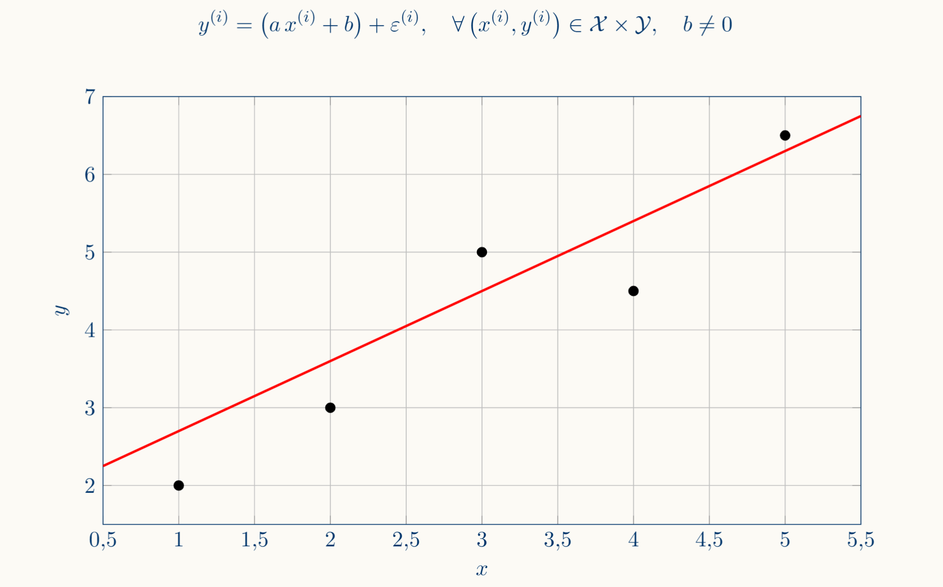
Thus, suppose we have $n$ observations, each observation is a pair $(x^{(i)},y^{(i)}) \in \mathcal{X} \times \mathcal{Y}$ where the output is roughly determined by the input, with some noise on top: $y^{(i)} = f(x^{(i)}) + \varepsilon^{(i)}$ (this is the affine relation we talked about above), then the linear regression is the decision to search only among affine maps as candidates for $f$:
1.2.1.3. Classification Models.
Before, we've introduced Regression models with Linear Regression but we will cover that topic more extensively later.
Now we are going to cover the Classification Model; we've already internalized the regression setup: you have a hypothesis $h : \mathcal{X} \to \mathcal{Y}$ that predicts a continuous response; $h$ is continuous at any point which only makes sense if $\mathcal{Y}$ is isomorphic to some subset of $\mathbb{R}^n : n \in\mathbb{N}$. Classification arises when this hypothesis is no longer continuous, in the sense that $\mathcal{Y}$ is a discrete set.
In regression we talked about an error approximation through the loss function $\ell$ which tries to predict how far the prediction is from the desired output in a geometric "metric" sense; you care about the magnitude of the error, how far you are. In classification, being $\mathcal{Y}:= \Set{1,…,k}$ there is no meaningful notion of "distance"; when you predict a wrong class in $Y$, there is no notion of nearness to the correct answer in the sense that class $1$ isn't any closer or much better than class $7$ when the desired output is class $3$; there are only right or wrong answers.
This collapses $\ell$ to the 0-1 loss, which counts misclassifications:
\[\ell(h(x),y) = \mathbf{1}[h(x) \ne y]\]In regression you minimize empirical risk with a continuous loss (squared error, absolute error), and the hypothesis class consists of functions $h: \mathcal{X} \to \mathbb{R}$. In classification you minimize empirical risk with a discrete loss (0-1 loss), and the hypothesis class consists of functions $h: \mathcal{X} \to \Set{1,…, k}$
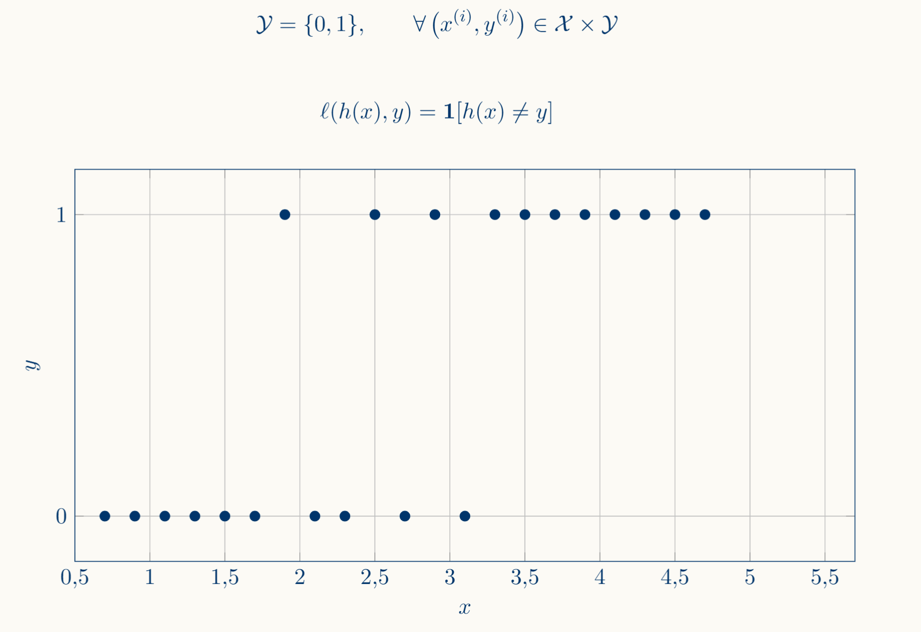
Then, basically, classification models force the machine to recognise previously labeled classes (by minimizing the error function) using the hypothesis $h$ over the input $x$ data and identifying it as some value of the discrete codomain $y$.
1.2.2. Unsupervised Learning. Clustering.
The idea on a high level is that, in contrast to supervised learning, the labeling of the output $y$ disappears; there are no wrong answers when applying the hypothesis on the data. The task for the algorithm is to find structures in the data; clusters.
In Classification there is a training set $\Set{(x_i,y_i)}_{i=1}^n$ where the labels $y_i$ were given by an oracle, in the sense that it is the desired output. Then, the task is to find a map that approximates $x \to y$ as much as possible. Observe that the categories exist before the algorithm starts the distinction.
Clustering inverts this relationship. The training set consists only of $\Set{x_i}_{i=1}^n$ (without labels). The task is to discover that there are groups at all, and to assign each point to one. The categories are not predefined; they emerge from the geometric or distributional structure of the data itself. The fundamental assumption behind clustering is that the data is not uniformly spread across $\mathcal{X}$, but concentrates around certain regions. Clustering algorithms formalize different notions of what "concentrate" means:
-
Centroid-based; structure means proximity to a representative point.
-
Density-based; structure means regions of high density separated by regions of low density.
-
Distributional; structure means the data was plausibly generated by a mixture and inference on the latent component assignments.
Each of these is a different inductive bias about what a "cluster" is.
The comparison is more subtle than "one has labels, the other doesn't."
The problem is ill-defined in a way classification is not.
-
In classification, given a loss function and a hypothesis class, the optimal classifier is a well-defined object (the Bayes classifier, the ERM solution, etc.).
-
In clustering, there is no unique "correct" partition, the answer depends on your notion of similarity, the number of clusters $k$ (often a hyperparameter you must choose), and the scale at which you look. Two entirely different clusterings of the same data can both be "valid."
2. Regression Model.
2.1. Linear Regression Overview.
Now, we are going to dive into the Linear Regression Model; this is the most widely used learning algorithm and many of the concepts used to explain it apply to other training algorithms.
Let's make clear that Linear Regression is an instantiation of what we call Supervised Learning, which is a training model that consists of first training the machine with previously labeled data $(x,y)$, where $x$ is called the input feature data and $y$ is the output target variable (the expected output). Also it is important to know that we have a finite number of training pairs $n$.
When you finish the training, you let the machine predict outputs for new unlabeled data.
Each training pair is reflected in a Cartesian coordinate system forming a cloud of points. As we said before, linear regression consists of the assumption that the relation between each pair is an affine transformation, or simply a line:
The notation $(x^{(i)},y^{(i)}) \in \mathcal{X} \times \mathcal{Y}$ refers to the fact that we are treating the i-th pair in the sample. Also, each pair is reflected in a table opposing $x$ and $y$ in an $n$-row table:
| pair | x | y |
|---|---|---|
| $1$ | $x^{(1)}$ | $y^{(1)}$ |
| … | … | … |
| $n$ | $x^{(n)}$ | $y^{(n)}$ |
2.2. Training the machine. Linear regression.
Remember that the training algorithm's job is to form a function $f$ with the provided training set such that the transformation of an input feature $x$ by $f$, the prediction; $f(x)=\hat{y}$, is approximated enough to the target $y$; the expected output; $\hat{y} \to y$.
As we said before, linear regression assumes that $f$ is represented as a straight line in the graph of the form:
\[\hat{y} = f_{w,b}(x) := wx + b : w,b \in \mathbb{R}\]It is worth noting that these parameters tell us how $\hat{y}$ is built from $x$:
-
$w$ represents how much $x$ contributes to $\hat{y}$; this will be clearer when the linear regression model for multiple variables gets introduced; $x$ and $w$ are vectors related in $f$ by the dot product. This way each $w_i \in w$ tells us how much the $x_i \in x$ feature contributes to the value of $\hat{y}$.
-
$b$ as well represents how much $y$ is independent of $x$ since it is a constant value not related to the input. Observe that when $x = 0$, then $\hat{y} = b$ exactly, showing that this is the value that separates $\hat{y}$ from any $wx$.
2.3. Cost Function.
2.3.1. Squared Error.
Until now, we established that linear regression is about a finite training set that is represented in a coordinate system. We want a line such that $y = wx + b$ represents well enough the relation between the points.
Let's now dive into what well enough means. Well enough means that it minimizes the error in the prediction; let's now see what we call error and how to measure it.
The most natural thing to measure is the residual: how far off is the prediction from the truth:
\[e^{(i)}= \hat{y}^{(i)} - y ^{(i)}\]So in intuitive terms, the thing we want to measure is $\displaystyle \sum_{i=1}^{n}e^{(i)}$, but positive and negative terms can cancel out and erase part of the information.
The two natural candidates to solve the problem, $\vert e^{(i)} \vert$ and the square $(e^{(i)})^2$; the reason why we decide to square is because it is differentiable at any point (we will understand this later); $\displaystyle \sum_{i=1}^{n}(e^{(i)})^2$
Now we take the average (so the cost doesn't scale arbitrarily with dataset size):
\[\displaystyle \frac{1}{n} \sum_{i=1}^{n}(e^{(i)})^2\]This is the Mean Squared Error. It gives you a single number that summarizes how badly the line misses the data on average and is essentially what we are measuring.
In practice you'll almost always see a factor of $\frac{1}{2}$ thrown in front:
\[J(w,b) := \frac{1}{2m} \sum_{i=1}^{m} \bigl(f_{w,b}(x^{(i)}) - y^{(i)}\bigr)^2\]This doesn't change which $(w,b)$ minimizes $J$ (it's just a positive constant scaling). It's there purely for convenience: when you take the derivative, the exponent $2$ comes down and cancels with the $\frac{1}{2}$, giving you cleaner gradient expressions.
2.3.2. Interpretation. Optimization Problem.
Let's observe that $J(w,b)=0$ means that every single squared residual is zero, which forces each prediction to coincide with the labeled value; $f_{w,b}(x^{(i)}) = y^{(i)} \ \ \forall (x^{(i)},y^{(i)}) \in P(x,y)$
As $J$ increases, the line deviates more. This way, $J$ defines an ordering on parameter pairs $(w,b)$ lower $J$ means a better-fitting line. Finding the best line is now a clean optimization problem; minimize $J$ over $(w,b) \in \mathbb{R}^2$.
One thing worth noting: $J$ being zero is typically impossible (or undesirable) with real data, since the data has noise. But the key property holds $J$ is non-negative, equals zero only at perfect fit, and increases monotonically with the aggregate deviation of predictions from targets.
3. Gradient Descent.
We just saw that, in linear regression model we assume that exists an affine transformation $f_{w,b}(x) := wx + b$ that makes a solid prediction over the labeled points $(x,y) \in \mathcal{X} \times \mathcal{Y}$. We also said that a way to measure how "solid" this line is, is to build our Cost Function, represented as: $J(w,b) = \frac{1}{2m} \sum_{i=1}^{m} \bigl(f_{w,b}(x^{(i)}) - y^{(i)}\bigr)^2$ and we establish it as an optimization problem over the $(w,b) \in \mathbb{R}^2$ that minimizes the $J$ value as much as possible.
Now, Gradient Descent taught us a way to consistently search for $(w,b)$ pairs.
3.1. Introducing the problem.
We have the Mean Squared Error; $J(\theta)$, which measures the average distance-error between the predicted values $\hat{y}$ and the labeled values $y$, and we want to find that parameter $\theta^*$ that minimizes that error.
For a simple system, for example a continuous one-variable function on a real segment, we would calculate $\nabla J(\theta) = 0$:
\[\nabla J(\theta) := \begin{pmatrix} \frac{\partial J}{\partial \theta_1}(\theta)\\ \frac{\partial J}{\partial \theta_2}(\theta)\\ \vdots\\ \frac{\partial J}{\partial \theta_n}(\theta) \end{pmatrix}\quad \underbrace{\implies}_{n=1} \quad \nabla J(\theta) = \frac{\partial J}{\partial \theta}(\theta) = \frac{dJ(\theta)}{d\theta} = J'(\theta) = 0\]But in the moment the parameter space grows, that closed-form solution either doesn't exist or becomes computationally prohibitive. An iterative method is needed.
3.2. Gradient Descent Algorithm.
Gradient Descent exploits one fundamental fact from calculus: the gradient $\nabla J(\theta)$ points in the direction of steepest ascent of $J$ at $\theta$, meaning that to "decrease" $J$ implies moving $\theta$ towards the opposite direction of $\nabla J$:
\[\theta^{(t+1)} := \theta^{(t)} - \alpha \,\nabla J(\theta^{(t)}): \alpha \in \mathbb{R}^+\]Where $\alpha$ is the learning rate and controls the step size.
This way, computing $\nabla_\theta J$ gives you a concrete vector that tells you how each parameter contributes to the error. In the sense that each component $\frac{\partial J}{\partial \theta_j}$ tells you how $J$ (the error) changes, let's keep in mind the image above, $\theta$ always advances from left to right, this means that:
-
If $\frac{\partial J}{\partial \theta_j} > 0$, then the function is ascending and is moving away from the minimum, $\theta$ has overshot the minimum to the right so subtracting a positive value $\alpha · \frac{\partial J}{\partial \theta}$ from $\theta$ nudges $\theta$ to the left, hence $J$ towards the minimum.
-
If $\frac{\partial J}{\partial \theta_j} < 0$, then the function is descending and is approaching the minimum, $\theta$ has the minimum in front, to the right, so subtracting a negative value $\alpha · \frac{\partial J}{\partial \theta}$ is like adding a positive one, nudging $\theta$ forward and hence $J$ towards the minimum.
So, the sign always corrects the direction in both cases.
It is worth noting that convexity matters. For linear regression, $J$ is convex, there's a single global minimum and gradient descent will find it (given a reasonable $\alpha$). For neural networks, $J$ is non-convex with many local minima and saddle points.
It is also worth noting that, as $J$ gets closer to the minimum, the derivative term gets smaller in absolute terms, meaning that the term subtracted from $\theta$ is smaller, so $J$ advances more slowly to the minimum as it gets closer through Gradient Descent.
Observe that applying this to our linear regression model:
\[J(w,b) := \frac{1}{2m} \sum_{i=1}^{m} \bigl(f_{w,b}(x^{(i)}) - y^{(i)}\bigr)^2 \implies \nabla J(w,b) := \begin{pmatrix} \frac{\partial J(w,b)}{\partial w} \\ \frac{\partial J(w,b)}{\partial b} \end{pmatrix}\]Where:
\[\begin{cases}\frac{\partial J(w,b)}{\partial w} =\frac{1}{m} \sum_{i=1}^{m} \bigl(f_{w,b}(x^{(i)}) - y^{(i)}\bigr)x \\ \frac{\partial J(w,b)}{\partial b} = \frac{1}{m} \sum_{i=1}^{m} \bigl(f_{w,b}(x^{(i)}) - y^{(i)}\bigr) \end{cases}\]1. Multiple Input Features.
In our previous notes, our input was a single feature $x \in \mathbb{R}$ and the linear regression imposes the hypothesis to be an affine transformation: $f_{w,b}(x):=wx + b$, with two parameters.
Now suppose each observation has $d$ input features instead of one. The $i$-th training example is no longer a scalar $x^{(i)}$, but a vector:
\[x^{(i)} = \begin{pmatrix} x^{(i)}_1 \\ x^{(i)}_2 \\ \vdots \\ x^{(i)}_d \end{pmatrix} \in \mathbb{R}^{d}\]Then, $w$ is also another vector, this can be seen as the complements of the features, so the affine transformation gets the form:
\[f_{w,b}(x) = w_1 x_1 + w_2 x_2 + \cdots + w_d x_d + b = \sum_{i=1}^d (w_ix_i) + b = w^\top x + b\]Let's observe that it is easier now to observe that each $w_i$ tells us how much $x_i$ contributes to $\hat{y} = f_{w,b}$ and how $b$, remaining a scalar, keeps maintaining the distance between $w · x$ and $\hat{y}$.
Let's now extend the vectorial product to simplify the expression by forming:
\[\tilde{x} = \begin{pmatrix} 1\\ x_1\\ \vdots\\ x_d \end{pmatrix},\qquad \theta = \begin{pmatrix} b\\ w_1\\ \vdots\\ w_d \end{pmatrix}\]And defining $f_{\theta}(\tilde{x}) = \theta^\top \tilde{x} = w^\top x + b$
Then, the cost function is:
\[J(\theta) = \frac{1}{2m} \sum_{i=1}^{m} \bigl(\theta^\top \tilde{x}^{(i)} - y^{(i)}\bigr)^2\]And the gradient is:
\[\nabla J(\theta) := \begin{pmatrix} \frac{\partial J}{\partial \theta_1}(\theta)\\ \frac{\partial J}{\partial \theta_2}(\theta)\\ \vdots\\ \frac{\partial J}{\partial \theta_n}(\theta) \end{pmatrix}\]Where:
\[\frac{\partial J}{\partial \theta_j} = \frac{1}{m} \sum_{i=1}^{m} \bigl(\theta^\top x^{(i)} - y^{(i)}\bigr) x_j^{(i)}\]So conceptually, multivariate linear regression is identical to univariate — you just have more components in the gradient. Every intuition from the previous post (sign correction, convexity, learning rate behavior) carries over unchanged.
2. Vectorization.
2.1. Mathematical concept.
Vectorization is a technique to compute the gradient of a multivariable regression model efficiently. At the cost function there are $n$ training examples, each a vector in $\mathbb{R}^{d+1}$. The direct implementation is a double loop over $n$ examples, and for each, loop over $d+1$ components to compute $\theta^\top \tilde{x}^{(i)}$. This is computationally terrible.
The key observation is that the entire training set can be packed into a single matrix.
\[X = \begin{pmatrix} (x^{(1)})^\top \\ (x^{(2)})^\top \\ \vdots \\ (x^{(m)})^\top \end{pmatrix} \in \mathbb{R}^{m \times (d+1)}\]And thus, the vector of all predictions can be defined as the following matrix product:
\[\hat{Y}= X \theta \in \mathbb{R}^m\]This way, the $i$-th entry $X \theta$ is exactly: $(x^{(i)})^\top \theta$, which is the prediction for the $i$-th example.
The cost function becomes:
\[J(\theta)=\frac{1}{2m}\vert \vert X \theta−Y \vert \vert^2\]The entire gradient computation is, this way, expressed as two linear algebra operations. This is particularly important in computation, since when you write a Python loop to compute $\sum_{i=1}^m (\theta^\top x^{(i)} - y^{(i)}) x_j^{(i)}$ for each $j$, every iteration has interpreter overhead, cache misses, and no parallelism.
When you write X.T @ (X @ theta - y) in NumPy, the actual work is dispatched to BLAS (Basic Linear Algebra Subprograms), highly optimized Fortran/C routines that exploit CPU vector instructions (SIMD: single instruction, multiple data), cache-aware memory access patterns, and sometimes multiple cores. The algorithmic complexity is the same $O(md)$, but the constant factor can differ by orders of magnitude.
2.2. Vectorization with python.
2.2.1. Python and C.
Python makes no assumptions at parse time about what type a variable holds. The price of that flexibility is paid per operation, every time. It is an interpreted, dynamically-typed language meaning that at runtime, every operation on every value requires the interpreter to inspect the object's type, resolve the appropriate method, perform type coercion if needed, and manage reference-counted memory, all before the actual arithmetic happens.
Also, Python represents every value as a heap-allocated object with a type pointer, a reference count, and the actual payload. When you store n floats in a Python list, you have a contiguous array of pointers, each pointing to a separate heap-allocated float object scattered across memory. The data is fragmented by design.
These two problems together mean that iterating over n numerical values in Python incurs $O(n)$ interpreter overhead, $O(n)$ pointer dereferences with poor cache locality, and $O(n)$ dynamic type dispatches, none of which contribute to the actual mathematical computation.
C (and Fortran) operate under a fundamentally different model. Types are resolved at compile time, values are stored inline in contiguous memory without metadata wrappers (often in the stack), and the compiled machine code operates directly on raw bytes with no interpreter mediating each instruction.
A loop over n doubles in C touches a flat buffer sequentially, which is exactly the access pattern modern CPUs and their cache hierarchies are optimized for. Furthermore, decades of work in numerical linear algebra (BLAS, LAPACK) have produced C/Fortran libraries that exploit hardware-level parallelism, SIMD instruction sets that process multiple floats in a single clock cycle. These libraries represent the practical floor of how fast a given computation can run on a given CPU.
2.2.2. Numpy.
NumPy stands for Numerical Python, is a C-backed Python library that provides an n-dimensional array object (ndarray) and a large collection of mathematical operations that act on these arrays. The key insight is that the ndarray is a contiguous block of homogeneous, typed memory (not a python list of python objects).
When you write np.array([1.0, 2.0, 3.0]), you get a flat buffer of 64-bit floats laid out sequentially in memory, with shape/stride metadata on top. This is essentially the same memory layout a C or Fortran program would use.
Python does have a math module, but it solves the function resolution problem not efficient computation. NumPy resolves this by moving the inner loop from Python to C. It provides a Python object (ndarray) that internally holds a flat, typed, contiguous buffer, the same memory layout a C program would use. When you call a NumPy operation, Python dispatches once to a compiled C routine, which then iterates over the raw buffer with no interpreter involvement per element. The cost model changes from $O(n)$ Python operations to $O(1)$.
2.2.3. Numpy basic usage.
2.2.3.1. Importing Numpy.
We can import Numpy to our repository with:
import numpy as np    # it is an unofficial standard to use np for numpy
import time
2.2.3.2. Vectors and Numpy arrays.
Vectors are ordered arrays of numbers. The number of elements in the array is often referred to as the dimension. The vector shown has a dimension of $n$.
The elements of a vector can be referenced with an index. In math settings, indexes typically run from $1$ to $n$. In computer science indexing will typically run from $0$ to $n-1$.
NumPy's basic data structure is an indexable, n-dimensional array containing elements of the same type (dtype). Let's observe that in maths and computation, the dimension is not the same.
The dimension or rank of a vector $v$ refers to the number of elements of the basis of the vector space $V : v \in V$ which essentially refers to the $n$ in $\mathbb{R}^n : V \simeq \mathbb{R}^n$ (informally speaking, the number of 'elements' of the vector).
In computer science, dimension refers to the number of indices in the array; the array has a shape, which refers to the number of elements per index, and a dimension, which is the number of indices. This way, an $n$-dimensional vector coincides with a $1$-D array of shape $n$.
numpy.array
Create an array.
In [28]: print(np.array([1,2,3,4]))
[1 2 3 4]
numpy.zeros
numpy.zeros, according to the documentation; return a new array of given shape and type, filled with zeros.
numpy.zeros(shape, dtype=None, order='C', *, device=None, like=None)
Parameters:
-
shape: int or tuple of ints
Shape of the new array, e.g., (2, 3) or 2.
-
dtypedata-type, optional
The desired data-type for the array, e.g., numpy.int8. Default is numpy.float64.
-
order{‘C’, ‘F’}, optional, default: ‘C’
Whether to store multi-dimensional data in row-major (C-style) or column-major (Fortran-style) order in memory.
-
devicestr, optional
The device on which to place the created array. Default: None. For Array-API interoperability only, so must be "cpu" if passed.
In order to show some examples, the ipython3 tool is being used:
In [16]: print(np.zeros(4)); print(np.zeros(4).shape);  print(np.zeros(4).dtype)
[0. 0. 0. 0.]
(4,)
float64
numpy.random.rand
Random values in a given shape. Create an array of the given shape and populate it with random samples from a uniform distribution over [0, 1).
In [25]: print(np.random.rand(4))
[0.62305938 0.22321443 0.71399    0.09377264]
In [28]: print(np.random.rand(4,2))
[[0.77512097 0.76052161]
 [0.32290935 0.05235408]
 [0.04702614 0.95376066]
 [0.27955549 0.92774067]]
numpy.arange
Return evenly spaced values within a given interval.
>>> print(np.arange(4))
[0 1 2 3]

In [16]: print(np.arange(2,4))
[2 3]

In [17]: print(np.arange(0,100,10))
[ 0 10 20 30 40 50 60 70 80 90]
2.2.3.3. Operation on vectors.
Let's explore some operation with the vectors.
Indexing
Elements of vectors can be accessed via indexing and slicing. NumPy provides a very complete set of indexing and slicing capabilities.
In [18]: print(np.arange(0,100,10)[2])
20
If we pass a 'minus' index, we access the slots from the opposite side:
In [18]: print(np.arange(0,100,10)[-2])
80
Slicing
Slicing creates an array of indices using a set of three values (start:stop:step). A subset of values is also valid.
In [23]: print(np.arange(100)[10:])
[10 11 12 13 14 15 16 17 18 19 20 21 22 23 24 25 26 27 28 29 30 31 32 33
 34 35 36 37 38 39 40 41 42 43 44 45 46 47 48 49 50 51 52 53 54 55 56 57
 58 59 60 61 62 63 64 65 66 67 68 69 70 71 72 73 74 75 76 77 78 79 80 81
 82 83 84 85 86 87 88 89 90 91 92 93 94 95 96 97 98 99]

In [22]: print(np.arange(100)[10:20])
[10 11 12 13 14 15 16 17 18 19]

In [26]: print(np.arange(100)[10:50:5])
[10 15 20 25 30 35 40 45]
Unary vector operations
Let's see how to operate with unary operations:
In [29]: print(-np.array([1,2,3,4]))
[-1 -2 -3 -4]

In [33]: print(np.sum(np.array([1,2,3,4]))) # Sum the components.
10

In [34]: print(np.mean(np.array([1,2,3,4]))) # Get the mean.
2.5

In [36]: print(np.array([1,2,3,4])**2) # Power to 2 the items of the list.
[ 1  4  9 16]
Vector element-wise operations
Most of the NumPy arithmetic, logical and comparison operations apply to vectors as well. These operators work on an element-by-element basis. For example:
\[c_i = a_i + b_i\]In [2]: print(np.array([1,2,3,4])+ -np.array([1,2,3,4]))
[0 0 0 0]
for this to work correctly, the vectors must be of the same size.
\[b_i = \alpha a_i\]In [3]: print(5*np.array([1,2,3,4]))
[ 5 10 15 20]
Vector dot product
Being $a,b \in V$, then we define the dot product of $a$ and $b$ as:
\[a·b = \sum_{i=1}^{n}a_ib_i\]The dot product multiplies the values in two vectors element-wise and then sums the result. Vector dot product requires the dimensions of the two vectors to be the same.
Without it we would have to implement a for loop to first perform $n$ products and then do the summation, but NumPy has the .dot method:
In [7]: print(np.dot(np.array([1,2,3,4]),np.array([1,2,3,4])))
30
Let's also perform the same operation through the two methods and see which of the two spends more time computing the code and verify if the efficiency of NumPy is worth it.
First, take a look over the following test file:
import numpy as np
import time

def my_dot(a, b):
    """
   Compute the dot product of two vectors

    Args:
      a (ndarray (n,)):  input vector
      b (ndarray (n,)):  input vector with same dimension as a

    Returns:
      x (scalar):
    """
    x=0
    for i in range(a.shape[0]):
        x = x + a[i] * b[i]
    return x


np.random.seed(1)
a = np.random.rand(10000000)  # very large arrays
b = np.random.rand(10000000)

tic = time.time()  # capture start time
c = np.dot(a, b)
toc = time.time()  # capture end time

print(f"np.dot(a, b) =  {c:.4f}")
print(f"Vectorized version duration: {1000*(toc-tic):.4f} ms ")

tic = time.time()  # capture start time
c = my_dot(a,b)
toc = time.time()  # capture end time

print(f"my_dot(a, b) =  {c:.4f}")
print(f"loop version duration: {1000*(toc-tic):.4f} ms ")

del(a);del(b)  #remove these big arrays from memory
The produced output is:
$ python3 test.py
np.dot(a, b) =  2501072.5817
Vectorized version duration: 14.1015 ms
my_dot(a, b) =  2501072.5817
loop version duration: 1158.4625 ms
2.2.3.4. Matrix and operation with matrices.
Matrices are two-dimensional arrays. The elements of a matrix are all of the same type.
In math settings, numbers in the index typically run from 1 to n. In computer science and these labs, indexing will run from 0 to n-1.
NumPy's basic data structure is an indexable, n-dimensional array containing elements of the same type (dtype). These were described earlier. Matrices have a two-dimensional (2-D) index [m,n].
Indexing
Matrices include a second index. The two indexes describe [row, column]. Access can either return an element or a row/column:
In [4]: a = np.arange(6).reshape(-1, 2) #Reshape allow to expand dimension
        print(f"a.shape: {a.shape}, \na= {a}")
a.shape: (3, 2),
a= [[0 1]
 [2 3]
 [4 5]]
3. Multiple Linear Regression.
Let's now extend the previously visited concepts and NumPy methods to build a Multi-Variable Linear Regression.
3.1. Defining the problem.
We will use the motivating example of housing price prediction. The training dataset contains three examples with four features (size, bedrooms, floors and age) shown in the table below.
| Size (sqft) | Number of Bedrooms | Number of floors | Age of Home | Price (1000s dollars) |
|---|---|---|---|---|
| 2104 | 5 | 1 | 45 | 460 |
| 1416 | 3 | 2 | 40 | 232 |
| 852 | 2 | 1 | 35 | 178 |
3.2. Writing our code.
First, we start by importing the necessary libraries:
import copy, math
import numpy as np
import matplotlib.pyplot as plt # Visualize 2D,3D functions
np.set_printoptions(precision=2)  # reduced display precision on numpy arrays
Now, we introduce our training set $\mathcal{X} \times \mathcal{Y}$, being:
- $\mathcal{X}\subset Size \times NBedrooms \times NFloors \times Age: \mathcal{X} := \begin{cases} (2104, & 5, & 1, & 45) \\ (1416, & 3, & 2, & 40) \\ (852, & 2, & 1, & 35) \end{cases}$
- $\mathcal{Y} \in Price^3: \mathcal{Y}:= (460, 232, 178)$
This data is introduced making use of following arrays:
X_train = np.array([[2104, 5, 1, 45], [1416, 3, 2, 40], [852, 2, 1, 35]])
y_train = np.array([460, 232, 178])
Let's observe that we built the following structure from our data:
Let's remember that our goal is to find $f: \mathcal{X} \to \mathcal{Y}: f(x) = y \ \ \forall (x,y) \in \mathcal{X} \times \mathcal{Y}$.
The linear regression model assumes that there exists an affine transformation that approximates $f$ closely enough, in other words $\exists (w,b) \in \mathbb{Q^4} \times \mathbb{Q}$ such that:
\[y = f(x) \simeq f_{w,b}(x) := w · x + b\]Thus, $w \in \mathbb{Q}^4$ is a vector of $4$ elements $(w_1,w_2,w_3,w_4 )$ where $w_i$ determines how much $x_i$ of $x \in \mathbb{Q}^4$ affects the $f_{w,b}(x)$ value and $b \in \mathbb{Q}$ is a scalar parameter. Thus, we can reformulate $f_{w,b}$ as:
\[f_{w,b}(x) := w · x + b = \sum_{i=1}^4 w_ix_i + b\]This function depends on parameters $w$ and $b$.
For demonstration, $w$ and $b$ will be loaded with some initial selected values that are near the optimal.
b_init = 785.1811367994083
w_init = np.array([ 0.39133535, 18.75376741, -53.36032453, -26.42131618])
In order to perform the operation we can use the .dot method of the NumPy module instead of crafting a for loop as we saw before:
def f(x, w, b):
    """
    single predict using linear regression
    Args:
      x (ndarray): Shape (n,) example with multiple features
      w (ndarray): Shape (n,) model parameters
      b (scalar):             model parameter

    Returns:
      p (scalar):  prediction
    """
    p = np.dot(x, w) + b
    return p
Now, let's model the cost function which measures the prediction error of $f_{w,b}$ for certain $w,b$ given by $\hat{y}^{(i)} := f_{w,b}(x^{(i)}) \simeq y^{(i)}$:
\[J(w,b):= \frac{1}{6}\sum_{i=1}^3(f_{w,b}(x^{(i)}) - y^{(i)})^2\]We can compute it by:
def J(X, y, w, b):
    """
    compute cost
    Args:
      X (ndarray (m,n)): Data, m examples with n features
      y (ndarray (m,)) : target values
      w (ndarray (n,)) : model parameters
      b (scalar)       : model parameter

    Returns:
      cost (scalar): cost
    """
    m = X.shape[0]
    cost = 0.0
    for i in range(m):
        f_wb_i = np.dot(X[i], w) + b           #(n,)(n,) = scalar (see np.dot)
        cost = cost + (f_wb_i - y[i])**2       #scalar
    cost = cost / (2 * m)                      #scalar
    return cost
We want to find $\theta := (w,b) : \displaystyle\min_{\theta \in \Theta} \ J(\theta)$ and we go through the Gradient Descent algorithm. We remember that this algorithm tries to find a local minimum for $J$ by leveraging one fundamental fact: $\nabla J$ points to the direction which maximizes $J$, thus, we have to perform a finite sequence of steps of the form:
\[\theta_{t+1} := \theta_t - \alpha \nabla J (\theta_ t)\]Where $\alpha$ is our learning rate.
Applying the formula above to our model, let's first unravel what $\nabla J$ is.
Being $\theta := (w_1,w_2,w_3,w_4,b)$, then, we define:
\[\nabla J(w,b) := \begin{pmatrix} \frac{\partial J}{\partial w_1}(w,b) \\ \frac{\partial J}{\partial w_2}(w,b) \\ \vdots \\ \frac{\partial J}{\partial b}(w,b) \end{pmatrix} : \begin{cases} \frac{\partial J}{\partial w_j}(w,b) := \displaystyle\frac{1}{3}\sum_{i=1}^3(f_{w,b}(x^{(i)}) - y^{(i)})x_j^{(i)} : j =1,2,3,4\\ \frac{\partial J}{\partial b}(w,b):= \displaystyle\frac{1}{3}\sum_{i=1}^3(f_{w,b}(x^{(i)}) - y^{(i)}) \end{cases}\]In order to compute the gradient, first, take the shape and craft the vector variable for each partial $\frac{\partial J}{\partial \theta}$:
m,n = X.shape           #(number of examples, number of features)
dj_dw = np.zeros((n,))
dj_db = 0.
Observe that in python m,n = X.shape is unpacking the dimension of the matrix $X$; also we are "initializing" to zero the partial vectors $dw$ and $db$.
Now, we feed each element of the vectors by mathematically computing the error and adding it to the vector entry, then divide the entry by $m$.
for i in range(m):
    err = (f(X[i], w, b)) - y[i]
    for j in range(n):
        dj_dw[j] = dj_dw[j] + err * X[i, j]
    dj_db = dj_db + err
dj_dw = dj_dw / m
dj_db = dj_db / m
The whole code would be:
def nablaJ(X, y, w, b): # Gradient.
    m,n = X.shape           #(number of examples, number of features)
    dj_dw = np.zeros((n,))
    dj_db = 0.

    for i in range(m):
        err = (f(X[i], w, b)) - y[i]
        for j in range(n):
            dj_dw[j] = dj_dw[j] + err * X[i, j]
        dj_db = dj_db + err
    dj_dw = dj_dw / m
    dj_db = dj_db / m

    return dj_db, dj_dw
Also, this gradient computation must be inserted within a routine to become an algorithm:
def gradient_descent(X, y, w_in, b_in, cost_function, gradient_function, alpha, num_iters):

    # An array to store cost J and w's at each iteration primarily for graphing later
    J_history = []
    w = copy.deepcopy(w_in)  #avoid modifying global w within function
    b = b_in

    for i in range(num_iters):

        # Calculate the gradient and update the parameters
        dj_db,dj_dw = gradient_function(X, y, w, b)

        # Update Parameters using w, b, alpha and gradient
        w = w - alpha * dj_dw
        b = b - alpha * dj_db

        # Save cost J at each iteration
        if i<100000:      # prevent resource exhaustion
            J_history.append(cost_function(X, y, w, b))

        # Print cost every at intervals 10 times or as many iterations if < 10
        if i% math.ceil(num_iters / 10) == 0:
            print(f"Iteration {i:4d}: Cost {J_history[-1]:8.2f}   ")

    return w, b, J_history #return final w,b and J history for graphing
Observe that the code above is just assembling the pieces we already crafted in a step-by-step mechanism that resembles our gradient descent algorithm. By parts:
-
First, we create some arrays to store the results and the modified data:
J_history = [] w = copy.deepcopy(w_in) #avoid modifying global w within function b = b_in -
Then, we establish a number of iterations for our gradient descent algorithm which will determine how close we get to the local minimum and inside the loop we perform the approximation of the algorithm:
  for i in range(num_iters):

  # Calculate the gradient and update the parameters
  dj_db,dj_dw = gradient_function(X, y, w, b)

  # Update Parameters using w, b, alpha and gradient
  w = w - alpha * dj_dw
  b = b - alpha * dj_db

  # Save cost J at each iteration
  if i<100000:      # prevent resource exhaustion
      J_history.append(cost_function(X, y, w, b))

  # Print cost every at intervals 10 times or as many iterations if < 10
  if i% math.ceil(num_iters / 10) == 0:
      print(f"Iteration {i:4d}: Cost {J_history[-1]:8.2f}   ")
We can find the whole code in the following repository.
4. Problems with gradient descent.
4.1. Introducing the problem.
Sometimes, having a cost function $J(\theta)$ and applying a correct learning rate $\alpha$ doesn't conclude in a smooth convergence on the local minimum. In practice, the gradient descent applies a single learning rate $\alpha$ to update all parameters simultaneously; as we know, the algorithm performs the assignments as:
\[w_i := w_{i} - \alpha \frac{\partial J}{\partial w_i}\]Let's observe that later, these new parameters, which are being updated in the same "proportion" $\alpha$, contribute to the next prediction, leading to the risk of creating disproportions between the features since each lives in its own range of values.
For example; in certain conditions, $x_1 \in[0,1] \wedge x_2 \in [0,50000] \implies \frac{\partial J}{\partial w_2} » \frac{\partial J}{\partial w_1}$ not because $w_2$ is further from its optimum, but simply because $x_2$ has a larger numerical range. So the same $\alpha$ is simultaneously too large for $w_2$ (causing oscillation or divergence) and too small for $w_1$ (causing painfully slow progress).
You're forced into a compromise: pick a tiny $\alpha$ that prevents divergence along the sensitive direction, at the cost of crawling along every other direction.
The fundamental issue is a mismatch between the structure of the problem (features at wildly different scales) and the structure of the algorithm (a single scalar learning rate applied uniformly). The algorithm has no mechanism to treat each parameter according to its own geometry.
4.2. Solution to the problem; Feature Scaling.
Feature scaling is a preprocessing step that normalizes the range of input features before running gradient descent. The core reason is geometric: it reshapes the loss surface to make optimization dramatically more efficient.
Let's see some forms to actually do this.
4.3.1. Feature Scaling method.
If we have a $n$ number of features in each range of values as:
\[x_i \in [m_i,M_i] \subset \mathbb{R}^+: i \in [n]\]Then a solution would be to divide each feature between the maximum value of the range before operating with it:
\[x_i':= \frac{x_i}{M_i}, m_i' := \frac{m_i}{M_i} \implies x_i' \in [m_i',1] \subset \mathbb{R}^+ : i \in [n]\]Suppose for example that $x_1 \in [300,2000],x_2 \in [0,5]$, then $x_1' \in [0.15,1], x_2 \in [0,1]$. Geometrically, we would pass from ellipses to something more circular, allowing the path to the local minimum on the surface to be more accessible.
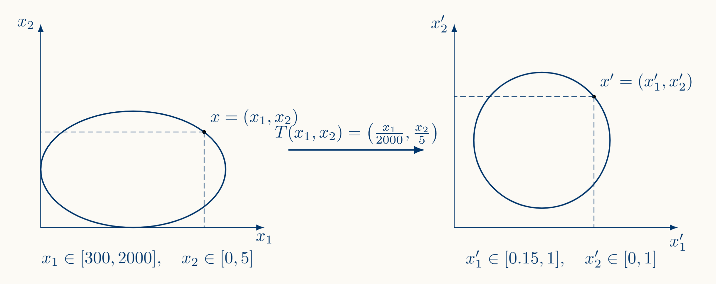
Note that the local minimum is accessible because the mapping $x \to x'$ we are applying here is an affine transformation; $x:= x'M +m$
4.3.2. Mean normalization.
There is also a variant of feature scaling called mean normalization; which is a feature scaling technique that transforms each feature so that it's centered around zero. Taking $x_i \in [m_i, M_i]$ then, mean normalization is the mapping given by:
\[x_i':=\frac{x_i - u_i}{M_i - m_i}: u_i:= \frac{1}{n}\sum_{j=1}^nx_i^{(j)}\]Where $u_i$ is the sample mean, the mean of the feature $i$ of all the samples $x^{(j)}$ in the training set.
The result is that each feature ends up roughly in $[-0.5,0.5]$ (assuming a reasonably uniform distribution), with mean approximately zero.
4.3.3. Z-Score (Standardization).
The Z-score normalization (also called standardization) transforms each feature as:
\[x_i' := \frac{x_i - u_i}{\sigma_i}\]Where $u_i$ still being the sample mean and $\sigma_i$ is the standard deviation which measures how spread out the values in a dataset are around their mean:
\[\sigma_i = \sqrt{\frac{1}{m} \sum_{j=1}^{m} \left(x_i^{(j)} - \mu_i\right)^2}\]For each data point you compute how far it is from the mean $(x_i^{(j)} - \mu_i)$, square that distance (so negative and positive deviations don't cancel), average all those squared distances, and then take the square root to bring the result back to the original units of the feature.
The core difference is in the denominator. Mean normalization divides by the range $(\max - \min)$, while Z-score divides by $\sigma$ which is more robust because it maps based on how far each feature is from the mean instead of simply generalizing the range for every feature. Geometrically, both aim at the same thing: making the level sets of $J(\theta)$ more isotropic (closer to spherical) so that $\nabla J$ points more directly toward the optimum. But Z-score does this more reliably because $\sigma$ is a better measure of the "typical spread" of a feature than the range is.
Thus; if the features are reasonably well-behaved (no extreme outliers, roughly symmetric), both methods give you similar results, the contours get reshaped about equally well, and gradient descent converges in roughly the same number of steps. The difference becomes significant when the data has heavy tails or outliers, where Z-score keeps the scaling stable while mean normalization can degrade.
5. Gradient Descent efficiency. Loss curve & Learning rate.
5.1. Introducing the concept.
Let's now suppose we have a good gradient descent algorithm and we want to run it and, as it runs, we want to be sure when the cost function $J$ converges to the local minimum.
For that purpose we build what we call the loss curve or training curve, which is simply the plot of your objective function $J(\theta^{(t)})$ (which in our case gets instantiated as the cost function) evaluated at each iterate $\theta^{(t)}$ against the iteration index $t$.
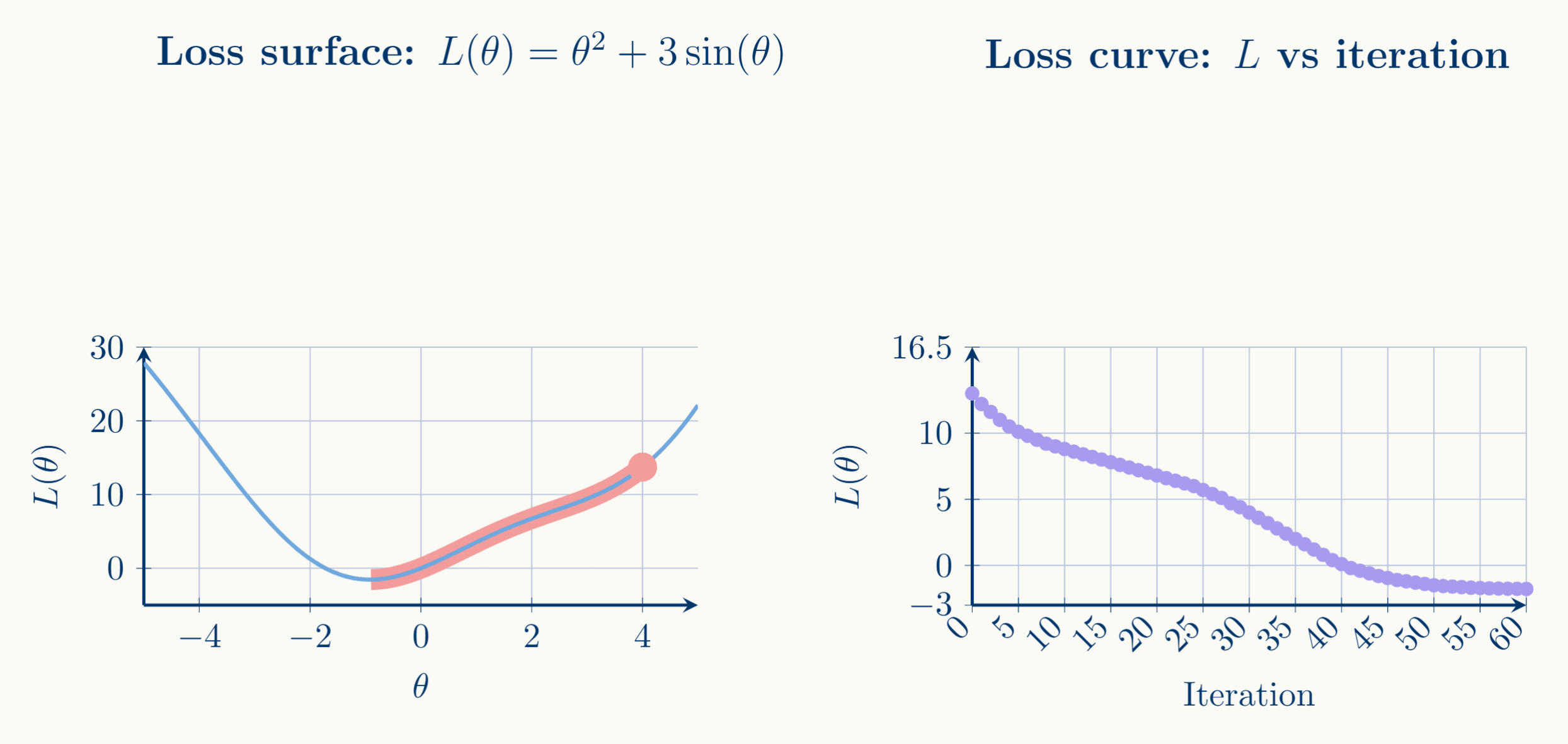
It's the most direct tool to determine whether gradient descent is converging, how fast it's converging, and whether your hyperparameters are well-chosen. As the picture shows, a healthy loss curve is monotonically decreasing and flattening toward an asymptote (our local minimum).
5.2. Formal setup.
Let $J : \mathbb{R}^n \to \mathbb{R}$ be your loss function and the gradient iteration:
\[\theta^{(t+1)}=\theta^{(t)}−\alpha \nabla J(\theta^{(t)})\]being $\alpha \in \mathbb{R}$ the learning rate. Then, we define the loss curve as the sequence:
\[\Big(J(\theta^{(t)})\Big)_{t=0}^\infty\]Assuming that $J$ is $\beta$-smooth, meaning $\nabla J$ is $\beta$-Lipschitz:
\[\vert \vert \nabla J(x) - \nabla J(y)\vert \vert \le \beta \vert \vert x-y\vert \vert \quad \forall x,y\]Conceptually, a function is β-Lipschitz when it has a bounded rate of change, it cannot "jump" too fast. Observe that if the gradient represents the "change ratio" of the function, how the function changes between two points is no greater than the metric between those same points (up to parameter factors). The change ratio grows (or decreases) proportionally per unit of distance in the domain (up to parameter factors).
Then, by the descent lemma it is:
\[J(\theta^{(t+1)}) \le J(\theta^{(t)}) - \alpha \left(1 - \frac{\beta \alpha}{2}\right) \vert \vert \nabla J(\theta^{(t)})\vert \vert^2\]The descent lemma gives you a guaranteed upper bound on how much a β-smooth function can deviate from its linear approximation. It's the formal reason why gradient descent works, it tells you that if you take a step in the direction of $-\nabla J(x)$, you can guarantee the function decreases, provided your step isn't too large.
Thus, this basically guarantees that the sequence we called loss curve smoothly decreases at each step until $\nabla J =0$
5.3. Choosing the learning rate.
As we set before, given a good gradient descent algorithm (a well-chosen learning rate $\alpha$) the results above tell us that the gradient descent algorithm should make the $J$ function decrease smoothly (descent lemma).
Whenever we see that our loss curve does not behave like that then mathematically we can ensure that the gradient descent algorithm is not well-formed.
A recommended good practice is to choose a small $\alpha$ and then increase it slowly. If this does not fix the loss curve, maybe there is a bug in the code.