2. Introduction to VectorSpaces
Algebra. Algebraic Structures. Actions. Vector Spaces. Affine Spaces. Vector as geometric objects: Arrows.
- Conceptual Approach: Algebra and Algebraic Structures.
- 1.1. Algebra as a discipline.
- 1.2. Algebraic Structures.
- 1.2.1. One operation algebraic structures.
- 1.2.2. Two operations algebraic structures.
- Vector spaces.
- 2.1. Actions. Algebraic Actions.
- 2.1.1. Definition.
- 2.1.2. Group's Action.
- 2.2. Field's action. Vector Space.
- 2.2.1. Definition.
- 2.2.2. Conceptually Approach.
- 2.3. Examples.
- 2.3.1. The n-tuple space.
- 2.3.2. The space of m x n matrices.
- 2.3.3. The space of functions from a set to a field.
- 2.3.4. The space of polynomial functions over a field K.
- 2.3.4.1. Introduction to polynomials.
- 2.3.4.2. Vector space of the polynomial functions over a field K.
- 2.4. Immediate Properties from vector spaces.
- 2.1. Actions. Algebraic Actions.
- Vector Spaces and Geometry.
- 3.1. Analytic Geometry: The affine space.
- 3.1.1. Definition.
- 3.1.2. Isomorphism by origin.
- 3.2. Vectors as geometric objects: Arrows.
- 3.2.1. Bound arrows. Vectors as arrows.
- 3.2.2. Equipolence class: Free vectors.
- 3.2.2.1. Appendix: Equivalence Class.
- 3.2.2.2. Vector equipolence.
- 3.1. Analytic Geometry: The affine space.
- Summary.
1. Conceptual Approach. Algebra, Algebraic Structures.
1.1. Algebra as a discipline.
Let's start by introducing what Algebra is. Algebra is the mathematical discipline in charge of the study of what operating with the elements of a set means: how items of a set are combined through an operation and what properties emerge from that context. It doesn't study the elements (like arithmetic would do) but the properties of the operations between them.
1.2. Algebraic Structures.
An algebraic structure is a set $(S, \Omega)$ where:
- $S \neq \varnothing$
- $\Omega$ is a collection of operations over $S$ (and maybe other sets as we will see) along with a sequence of rules called axioms that these operations satisfy.
This is the minimal basic item of study in algebra; a finite number of operations over a set defined by axioms. Our task is to comprehend how these operations behave through the axioms, applying classical logic.
In the previous section we already provided an introduction to algebraic structures through the number sets and then introduced a solid idea of the group and then the field. Our objective was to present a formalization about linear equations over a field.
We can review and develop the ideas presented in the Linear Equation section to understand the natural progression and the algebraic structures towards the vector space.
1.2.1. One operation algebraic structures.
Let $G := (S, \Omega) : \Omega := \Set{\star}$, where $\star : S \times S \to S$ is an internal operation (a function).
Then we define:
-
$G$ (or $S$ by default) is said to be a Magma if $\star$ only verifies the closure property:
- $a \star b \in S \ \ \forall a,b \in S$ (Closure)
Observe that this structure is the minimal one, and his only property is forced by $\star$ definition.
-
$G$ is a semigroup if it also verifies associativity:
- $a \star b \in S \ \ \forall a,b \in S$ (Closure)
- $(a \star b) \star c = a \star (b \star c) \ \ \forall a,b \in S$ (Associativity)
-
A monoid is a semigroup that also has the identity element $e \in S$ relative to $\star$ verifying:
- $a \star b \in S \ \ \forall a,b \in S$ (Closure)
- $(a \star b) \star c = a \star (b \star c) \ \ \forall a,b \in S$ (Associativity)
- $ \exists e \in S \ \ \forall a \in S : e \star a = a \star e = a$ (Identity)
-
Now we enter the comfort zone; a Group is a monoid which verifies the existence of an inverse for each item in $S$:
- $a \star b \in S \ \ \forall a,b \in S$ (Closure)
- $(a \star b) \star c = a \star (b \star c) \ \ \forall a,b,c \in S$ (Associativity)
- $ \exists e \in S \ \ \forall a \in S : e \star a = a \star e = a$ (Identity)
- $\forall a \in S \ \ \exists a' \in S : a \star a' = a' \star a = e$ (Inverse)
Let's observe that each axiom lets us do something new in the structure; each new rule is a new capability based on the defining of invariants along the structure;
-
The closure guarantees internal compositions; the belonging of any composition to $S$ remains constant.
-
The associativity guarantees order-independence as long as the direction in the composition remains the same, meaning that $(a\star b) \star c$ and $a\star (b \star c)$ are the same object in the sense that we can talk about $a\star b \star c$ to refer to any of them, no matter what you compose first.
-
The existence of the identity guarantees the existence of a way to operate that does nothing, concreted in an element of $S$ called the identity. The composition of $e$ with any item of $S$ in any direction remains constant and is the very same item.
-
The existence of the inverse makes use of the identity to guarantee a way to operate that lets you reverse the operation. The composition of any item with its inverse in any direction remains constant and is the identity.
Observe that these are the main invariants in operations because these are the smallest subset of rules that allow you to define constraints about some elements (equations) and comfortably operate to isolate them in order to fully understand what that constraint is equivalent to and what a valid item is.
Suppose there is an interest in finding the relation between two elements $a,b \in S$, this is, $b$ is the composition of $a$ with some other element $x \in S$ which we are going to call the unknown: $a \star x = b$. Now, let's observe:
\[a^{-1} \star (a \star x) = a^{-1} \star b\]Step by step, the closure axiom asserts that $a^{-1} \star (a \star x) = a^{-1} \star b \in S$ and the proposal makes sense; the associativity establishes that $a^{-1} \star (a \star x) = a^{-1} \star a \star x= (a^{-1} \star a) \star x$, or that we can choose the order of the composition as we please. Then, the identity and the inverse cooperate together to simplify the expression; the inverse makes $a$ disappear, it substitutes it for the identity and the identity composed with any other item is that other item, thus:
\[a^{-1} \star (a \star x) = (a^{-1} \star a) \star x = e \star x = x = a^{-1} \star b\]These four invariants are summarized in the idea of group.
This idea of group can be extended by introducing the commutativity which defines the composition under direction as an invariant:
\[a \star b = b \star a \ \ \forall a,b \in S\]This allows reorganizing, making the simplification of expressions even more comfortable.
1.2.2. Two operations algebraic structures.
Until now, we've defined an algebraic structure that contemplates only one operation; let's now introduce algebraic structures with two operations.
Rings
First, the rings; a ring is a triple $(K,+,\ ·)$ such:
- $(K,+)$ is a group and introduces the four properties seen above.
- $(K, \ ·)$ is a monoid, it drops the existence of the inverse for any element of $R$.
-
$+$ and $·$ relates themselves by the distributive law:
\[a(b+c) = ab + ac \wedge (b+c)a = ba + ca\]We say both operations are compatible.
The ring introduces the second operation in a soft way; hanging on the existence of the inverse allows it to fit in many well-studied structures such:
-
Integers ring; $(\mathbb{Z},+, \ ·)$, where for example $\forall a ( a \in \mathbb{Z} \wedge a \neq \pm 1 \implies a^{-1} \notin \mathbb{Z})$.
-
Polynomial ring; with coefficients in a field $F$; $F[x]$ is a ring but not a field. For instance, $x$ has no multiplicative inverse:
$\forall q \in F[x] \setminus {0} \ \deg(x \cdot q) = 1 + \deg(q) \geq 1 \neq 0 = \deg(1)$
So the equation $x \cdot q = 1$ has no solution in $F[x]$
-
Matrix ring; we've already seen that $(M_n(F)\setminus 0, \ ·)$ has no inverse for every element of $M_n(F)$; remember that we already saw that not every matrix is invertible, only those row-equivalent to the identity $I_n$
The mathematical world is full of structures with two operations where division fails.
Field
Then the concept of the field can be thought as an extension of the ring where each element has an inverse for the product operation except the zero element.
However, we want to present another perspective of a field.
Above we built step by step from the smallest algebraic structure Magma to the Group and his four axioms and we conclude the importance of such structure was that it allows to present and solve equations:
\[a \star x = b \iff x = a^{-1} \star b\]Then, the field $K$ aims to extend the same idea for two operations departing from the group structure. This means that a field is a triple $(K,+, \ ·)$ such:
- $(K, +)$ is an abelian group.
- $(K \setminus \Set{0}, \ ·)$ is an abelian group.
- $+$ and $·$ are compatible.
- $1 \neq 0$
This basically means that the field intends to be the structure in which equations can be defined and solved in two operations simultaneously; the motivation was to build an algebraic framework for common arithmetic operations in $\mathbb{R}, \mathbb{Q},…$ and other common fields.
2. Vector spaces.
Before, we've seen a set of axioms that rule how a set of operations $\Omega$ behaves in a non-empty set $K$. We extend this concept to two sets $(K,V)$ where $K$ is a field and $V$ is a group and both are related by a field-action.
Let's dive into this.
2.1. Actions. Algebraic Actions.
2.1.1. Definition.
First, let's define what an action is. Let $A$ and $S$ be two sets, then we define an action as a function:
\(\varphi: A \times S \to S\) \(\ \ \ \ \ \ \ (a,s) \to s\)
It grabs two elements, one from $A$ and another from $S$ and it maps it to a third element from $S$.
As defined, this function doesn't have any interest at all; it becomes interesting when $\varphi$ respects the structure of $A$; this way it is said that an action transforms $S$ using $A$'s algebraic structure.
2.1.2. Group's Action.
Group's action
Consider again $(G,S,\varphi)$ such that $\varphi : G \times S \to S$, let's suppose now that $G$ is a group for some internal operation $\star : G \times G \to G$.
In this context, we impose two rules $A1$, $A2$ over $\varphi : A \times S \to S$. In total, the triple $(G,S,\varphi)$ satisfies:
-
Closure: $\varphi(a,s) \in S \ \ \forall a \in G, s \in S$, forced by $\varphi$ definition.
-
(A1) Identity: Be $e \in G$ the identity on $G$ then we require: $\varphi(e,s) = s \ \ \forall s \in S$
Meaning that the $G$'s identity doesn't move anything through $\varphi$.
-
(A2) Associativity: $\varphi(a,\varphi(b,s)) = \varphi(a \star b,s) \ \ \forall a,b \in G, s \in S$
Observe that this resembles the order invariant we talked about in groups; as long as the direction of the composition remains still ($a \to b \to s$) it doesn't matter the order in which you perform these compositions.
Composing $b$ with $s$ through $\varphi$ and then this with $a$ is the same that "multiply" $a \star b$ in $G$ and then compose it with $s$ through $\varphi$. Check that if we write $a \star b = ab \wedge \varphi(a,s) = a\ ·s$ then, the rule above states that:
\[a \ ·(b \ ·s) = (ab)\ ·s \ \ \forall a,b \in G, s \in S\]And it appears more familiar.
-
Inverse: Observe this is not labeled as an axiom because it can be deduced from the two above but is included from pedagogic reasons.
The idea of the inverse on a group intends to formalice the idea of revert a composition or go back. Thus, we are looking to demonstrate that, calling $\varphi_a(s) = \varphi(a,s)$
\[\forall \varphi_a \ \exists \varphi^{-1}_{a} \ \forall s \in S: \varphi_a(\varphi^{-1}_{a}(s)) = \varphi^{-1}_{a}(\varphi_a(s)) = s\]Let's take $x = a^{-1}$ and observe that applying $A2$, $A1$ and the existence of the inverse in $G$ we get:
\[a^{-1} \ ·(a \ · s) = (a^{-1}a) \ · s = e \ · s = s\] \[a \ · (a^{-1} \ · s) = (aa^{-1}) \ · s = s\]Meaning that $\varphi^{-1}_{a}= \varphi_{a^{-1}} \ \ \forall a \in G$.
Thus, this four properties makes that the triple $(G,S,\varphi)$ behaves like a group in the sense that we can define and solve equations over the elements of $S$ which remember, initially wasn't a group:
\[\varphi_a(x) = s \iff x = \varphi_{a^{-1}}(s)\]Meaning that we can treat the elements of $S$ as elements over which we can define constraints, relations, etc.
Although, it is worth remembering that $S$ is not a group and neither is the triple $(G,S, \varphi)$; what $S$ has acquired through $\varphi$ is a family of reversible parametrized transformations by the group $G$. It is a way to use $G$ in order to study $S$.
2.2. Field's action. Vector Space.
2.2.1. Definition.
Now consider again a triple $(K,V,\ ·)$, where $K$ is a field and $V$ is an abelian group and $·: K \times V \to V$ is a field's action.
As we said before this action respects the algebraic structure of $K$, which remember; is a combined abelian group over two different compatible operations, by forcing the following axioms:
- M1: $1_K \ · v = v$. The identity over the product doesn't transform anything.
- M2: $\alpha \ · (\beta \ · v) = (\alpha \beta) \ · v \ \ \forall \alpha, \beta \in K, v \in V $. associativity resemblance, order-independence while direction stays still.
- D1: $\alpha \ · (u + v) = \alpha \ · u + \alpha \ · v \ \ \forall \alpha \in K, u, v \in V $. Compatibility between $·$ and $+$ in $V$.
- D2: $(\alpha + \beta) \ · v =\alpha \ · v + \beta \ · v \ \ \forall \alpha, \beta \in K, v \in V$. Compatibility between $·$ and $+$ in $K$.
This four axioms plus the four axioms of the group $V$ gives us the eight axioms of the vector space $(K,V, \ ·)$.
2.2.2. Conceptually Approach.
This time, a field's action over a group doesn't intend to give an algebraic structure to $V$; instead it provides, through $K$, a uniform deformation mechanism. The arithmetic system of $K$ as a field is used to perform richer algebraic manipulations on $V$ as a group.
$·: K \times V \to V$ gives to $V$ a parametric scaling mechanism through $(K,+, \ ·)$ which, ultimately, allows a coherent way to perform linear combinations on the elements of $V$.
Let's dive into "scaling", "linear" and "linear combination" terms in order to understand what this introduction means.
Scaling.
Scaling is about relating $V$'s elements using $K$'s elements as mediators. The term "scalar" comes from scale; changing the size without changing the essential nature of the object.
Then, being $u,v \in V$ and $\alpha \in K : \alpha \neq 0$, when we say that $u = \alpha \ · v$, we are really saying $u$ is obtained from $v$, keeping its structural information since, thanks to $K$ being a field and $·$ respecting $K$'s properties, we can revert this operation and go back from $u$ to $v$. Let's see that by $M2$ and $M1$ we can guarantee the existence of some $\beta \in K$ such that $\beta \ · u = v$. Take $\beta = \alpha ^{-1}$ and:
\[\alpha^{-1} \ · u = \alpha^{-1} \ · (\alpha \ · v) \underbrace{=}_{M2} (\alpha^{-1} \alpha) \ · v = (1_K) \ · v \underbrace{=}_{M1} v\]In this context we say that $u$ and $v$ are proportional. Specifically, there exists an entire family of elements to which $u$ is proportional: $\Set{\alpha v : \alpha \in K \wedge \alpha \neq 0} \subseteq V$.
Linear & Linear Combinations.
Linear refers to independent contributions of several parts which do not interfere between them.
In this case, a linear combination is the minimal operation that takes place in the triple $(K,V, \ ·)$; independent contribution of proportional components of $V$.
Is the most general way to combine while respecting the principle of independent contributions:
\[\alpha v + \beta u: \alpha , \beta \in K \ \ u, v \in V\]Observe that $D1$ and $D2$ guarantee that $K$ and $V$ respect this object on $(K,V,\ ·)$.
Vector Space
Thus, $(K,V, \ ·)$ is the algebraic environment where a set of objects can be combined by independent contributions weighted by a field. A field's action is the mechanism that imports the arithmetic of $K$ as a system of intensities applicable to the elements of $V$.
A vector space is nothing but, conceptually, a functional linear combination system and his elements are called vectors.
Vectors
Thus, vectors are elements of an algebraic structure called vector space whose elements relate through linear combinations verifying the eight axioms presented before.
Being the vector space an algebraic structure means that vectors (and vector spaces) are nothing; as we said at the start of these very notes, algebra cares about how to operate and the properties that emerge from some defined operable structure.
In other words; vectors are the elements of an abelian group $V$ on which a field $K$ acts through a "deformation" mechanism. This action, the combination or composition of these deformed elements of $V$, is what we call linear combinations: weighted sums where each element of $V$ contributes with an intensity set by $K$.
The corollary from this assertion is that what really matters is that there are objects (matrices, polynomials, arrows, etc.) that, with the right operations, verify the vector space axioms; thus, they are vectors and all the machinery defined around them works also for these objects.
2.3. Examples.
Let's see a few mathematical objects that algebraically behave as vector spaces.
2.3.1. The n-tuple space.
Consider $F$ a field, then the algebraic structure $(F^n,+)$ with the addition behaving as:
\[+: F^n \times F^n \to F^n \mid x + y := \begin{pmatrix}x_1 + y_1\\ \vdots \\ x_n+y_n\end{pmatrix} \in F^n\]Observe that the properties of the abelian group $(F,+)$ expand to $(F^n,+)$ so this is also an abelian group.
Thus, defining the function defined as:
\(· : F \times F^n \to F^n\) \((\alpha, \begin{pmatrix}x_1 \\ \vdots \\ x_n\end{pmatrix} ) \to \begin{pmatrix}\alpha x_1 \\ \vdots \\ \alpha x_n\end{pmatrix}\)
Verifies the field's action axioms:
-
M1: $1 \ · \begin{pmatrix}x_1 \ \vdots \ x_n\end{pmatrix} = \begin{pmatrix}1x_1 \ \vdots \ 1x_n\end{pmatrix} = \begin{pmatrix}x_1 \ \vdots \ x_n\end{pmatrix} \ \ \forall x \in F^n$
-
M2: $\alpha \ ·( \beta \ · \begin{pmatrix}x_1 \ \vdots \ x_n\end{pmatrix}) = \alpha \ · \begin{pmatrix}\beta x_1 \ \vdots \\beta x_n\end{pmatrix} = \begin{pmatrix}\alpha \beta x_1 \ \vdots \\alpha \beta x_n\end{pmatrix} = (\alpha \beta) \ · \begin{pmatrix}x_1 \ \vdots \ x_n\end{pmatrix} \ \ \forall \alpha, \beta \in F, x \in F^n$
-
D1:
\[\alpha \ · (\begin{pmatrix}x_1 \\ \vdots \\ x_n\end{pmatrix} + \begin{pmatrix}y_1 \\ \vdots \\ y_n\end{pmatrix}) = \alpha \ · \begin{pmatrix}x_1 +y_1 \\ \vdots \\ x_n + y_n\end{pmatrix} = \begin{pmatrix}\alpha (x_1 + y_1) \\ \vdots \\ \alpha (x_n + y_n)\end{pmatrix} = \begin{pmatrix}\alpha x_1 + \alpha y_1\\ \vdots \\ \alpha x_n + \alpha y_n\end{pmatrix}\] \[= \begin{pmatrix}\alpha x_1 \\ \vdots \\ \alpha x_n\end{pmatrix} + \begin{pmatrix}\alpha y_1 \\ \vdots \\ \alpha y_n\end{pmatrix} = \alpha \ · \begin{pmatrix}x_1 \\ \vdots \\ x_n\end{pmatrix} + \alpha \ · \begin{pmatrix}y_1 \\ \vdots \\ y_n\end{pmatrix} \ \ \forall x,y \in F^n, \alpha \in F\] -
D2:
\[(\alpha + \beta)\ · \begin{pmatrix}x_1 \\ \vdots \\ x_n\end{pmatrix} = \begin{pmatrix}(\alpha + \beta)x_1 \\ \vdots \\ (\alpha + \beta)x_n\end{pmatrix} = \begin{pmatrix}\alpha x_1 + \beta x_1 \\ \vdots \\ \alpha x_n + \beta x_n\end{pmatrix} = \begin{pmatrix}\alpha x_1 \\ \vdots \\ \alpha x_n\end{pmatrix} + \begin{pmatrix}\beta x_1 \\ \vdots \\ \beta x_n\end{pmatrix}\] \[= \alpha \ · \begin{pmatrix}x_1 \\ \vdots \\ x_n\end{pmatrix} + \beta \ · \begin{pmatrix}x_1 \\ \vdots \\ x_n\end{pmatrix}\]
Thus, the triple $\big(F,(F^n,+), \ · \big)$ satisfies:
- $F$ being a field.
- $(F^n,+)$ an abelian group.
- $(\ ·)$ is a field's action (an action satisfying $M1,M2,D1,D2$ axioms).
And is a vector space.
Observe that, as a special case, $(\mathbb{R},(\mathbb{C}^n,+), \ ·)$ is a vector space.
2.3.2. The space of m x n matrices.
Let's consider the set $M_{m \times n}(F) = F^{m \times n}$ with
\[+: F^{m \times n} \times F^{m \times n} \to F^{m \times n}\] \[(a_{ij}) + (b_{ij}) := \big((a_{ij} + b_{ij})_{ij} \big)\in F^{m \times n}\]Observe that again addition in $F^{m \times n}$ is extended from $(F,+)$ which is an abelian group so $(F^{m \times n},+)$ is also an abelian group, the argument is the same, addition in $F^{m \times n}$ are $mn$ additions on $F$.
Also, consider the action:
\(· : F \times F^{m \times n} \to F^{m \times n}\) \((\alpha, (a_{ij}) ) \mapsto (\alpha a_{ij})\)
Observe that:
-
M1: $1 \ · (a_{ij}) = (1 a_{ij}) = (a_{ij}) \ \ \forall (a_{ij}) \in F^{m \times n}$
-
M2: $\alpha \ · (\beta \ · (a_{ij})) = \alpha \ · (\beta (a_{ij})) = (\alpha \beta (a_{ij})) = (\alpha \beta) \ · (a_{ij}) \ \ \forall \alpha, \beta \in F, (a_{ij}) \in F^{m \times n}$
-
D1: \(\alpha \ · ((a_{ij}) + (b_{ij})) = \alpha \ · \big((a_{ij} + b_{ij})_{ij} \big) = \big(\alpha (a_{ij} + b_{ij})_{ij} \big) = \big(((\alpha a_{ij}) + (\alpha b_{ij}))_{ij} \big)\)
\[= (\alpha a_{ij}) + (\alpha b_{ij}) = \alpha \ · (a_{ij}) + \alpha \ · (b_{ij}) \ \ \forall \alpha \in F, (a_{ij}),(b_{ij}) \in F^{m \times n}\] -
D2:
\[(\alpha + \beta) \ · (a_{ij}) = (((\alpha + \beta)a_{ij})_{ij}) = ((\alpha a_{ij} + \beta a_{ij})_{ij}) = (\alpha a_{ij}) + (\beta a_{ij}) \ \ \forall \alpha, \beta \in F, (a_{ij})\in F^{m \times n}\]
This way, $F$ is a field, $(F^{m \times n},+)$ is an abelian group and $( \ ·)$ is a field's action of $F$ over $(F^{m \times n},+)$.
Thus, $\big(F,(F^{m\times n},+), \ · \big)$ is a vector space.
Let's observe that, despite we already touched some operation properties from the addition and product of matrix, the fact that this set is a vector space finish refining the details of both operations and how they related them selves.
2.3.3. The space of functions from a set to a field.
Consider now some field $K$ and some set $S \neq \varnothing$, then, remember that being $f : S \to K$ a function, this gets identified with its graph $f \subseteq S \times K : (\forall s \in S \ \exists ! \alpha \in K \mid (s,\alpha) \in f)$, meaning that a function is a relation in which every element of the domain has a unique image through $f$.
Then, the set of all the relations from $S$ to $K$ that are applications is:
\[K^S := \Set{f \in \mathcal{P}(S \times K) \mid \forall s \in S \ \exists ! \alpha \in K : (s,\alpha) \in f}\]In this context, we agree on the notation $f(s) = \alpha \iff (s,\alpha) \in f$, then let's call:
\[f = \Set{(s,f(s)) \mid s \in S}\]This is the set of all the functions from $S$ to $K$ and define an addition over $K^S$ elements as:
\[+ : K^S \times K^S \to K^S \mid (f,g) \mapsto f+g:= \Set{(s,f(s) + g(s)) \mid s \in S}\]Observe that, due to the closure in $(K,+)$ we have that $f(s) + g(s) \in K$, so $f+g \in K^S$. Or simply, abreviate it as the formulation: $(f+g)(s) = f(s) + g(s)$.
The addition definition again gets defined directly in terms of the addition in $K$, so $(K^S,+)$ is an abelian group. Being the neutral element and the inverse defined as:
\[i := \Set{(s, 0_K) \mid s \in S}\] \[-f := \Set{(s, -f(s)) \mid s \in S}\]Also, define the action:
\[· : K \times K^S \to K^S \mid (\alpha, f) \mapsto \alpha \ · f := \Set{(s,\alpha f(s)) \mid s \in S}\]And check that satisfies the field's action axiom:
-
M1: $1 \ · f = \Set{(s,1 f(s)) \mid s \in S} = \Set{(s,f(s)) \mid s \in S} = f$
-
M2:
\[\alpha \ ·(\beta \ ·f ) =\alpha \ · \Set{(s,\beta f(s)) \mid s \in S} = \Set{(s,\alpha \beta f(s)) \mid s \in S}\] \[= (\alpha \beta) \ · \Set{(s, f(s)) \mid s \in S} = (\alpha \beta) \ ·f\] -
D1:
\[\alpha \ · (f + g) = \alpha · \Set{(s, f(s) + g(s)) \mid s \in S} = \Set{(s,\alpha f(s) + \alpha g(s)) \mid s \in S}\] \[= \Set{(s,\alpha f(s)) \mid s \in S} + \Set{(s,\alpha g(s)) \mid s \in S} = (\alpha \ · f) + (\alpha \ · g)\] -
D2:
\[(\alpha + \beta) \ · f =(\alpha + \beta) \ · \Set{(s, f(s)) \mid s \in S} = \Set{(s,(\alpha+\beta) f(s)) \mid s \in S}\] \[=\Set{(s,\alpha f(s)+\beta f(s)) \mid s \in S}= \Set{(s,\alpha f(s)) \mid s \in S} + \Set{(s,\beta f(s)) \mid s \in S}\] \[= (\alpha \ · f)+ (\beta \ · f)\]
Thus, $( \ ·)$ is a field's action and $(K,(K^S,+),\ · )$ is a vector space.
2.3.4. The space of polynomial functions over a field K.
2.3.4.1. Introduction to polynomials.
A polynomial is, elementally, the simplest algebraic expression that can be formed by combining an indeterminate with itself along with scalars of a field $K$ using addition and multiplication operations.
\[\sum_{i=0}^n \alpha_i x^i = \alpha_0 + \alpha_1 x \cdots + \alpha_n x^n\]The concept of polynomial function emerges when you try to evaluate the expression on entities from an evaluation domain.
Note that we deliberately used indeterminate instead of unknown, since this last one resembles the scalars of a field, but in a polynomial function, usually, the domain can be more than scalars, it can be tuples, matrices, or even other polynomials.
In summary, a polynomial is a generic presentation of a finite sequence of operations over a single object with itself along with two predefined operations.
Vector space of the polynomial functions over a field K
Then let's consider a field $K$ and the set:
\[\operatorname{Pol}(K, K) := \left\{\, f \in K^K \ \middle|\ \exists n \in \mathbb{N}_0,\ \exists (\alpha_0, \ldots, \alpha_n) \in K^{n+1} : \forall s \in K,\ f(s) = \sum_{i=0}^{n} \alpha_i\, s^i \,\right\}\]Let's consider the same operations $+$ and $·$ than in the example before. Let's observe that:
-
$\boldsymbol{0} \in Pol(K,K)$, since the function $f (s) = 0 = \sum_{i=0}^n 0 s^i\ \ \forall s \in S$ have a polynomial form.
-
$f(s) + g(s) = (f+g)(s) = \sum_{i=0}^n (\alpha_i + \beta_i)s^i \in Pol(K,K) \ \ \forall f,g \in Pol(K,K)$, so the addition is closed on $Pol(K,K)$.
-
$ \forall f (-f \in Pol(K,K))$, just consider: $f(s) = \sum_{i=0}^{n} \alpha_i\, s^i$ other $g(s) = -(f(s)) = - (\sum_{i=0}^{n} \alpha_i\, s^i)$, then, is obvious that $(f + g)(s) = (g + f)(s) = \boldsymbol0$
Thus, we've just demonstrated that $(Pol(K,K),+)\leq (K^K,+)$; the abelian condition comes from commutativity on $(K,+)$, so $(Pol(K,K),+)$ is an abelian group.
Observe that $\alpha \ · f \in Pol(K,K) \ \ \forall f \in Pol(K,K)$, meaning that it does have sense to define the action $· : Pol(K,K) \to Pol(K,K)$ as a subfunction of $· \in \mathcal{P}(K^K \times K^K)$ defined above. Thus the properties of the field's action $·$ described above already applies to $Pol(K,K)$ since is a subset of $K^K$.
Thus, the triple $(K,Pol(K,K),\ ·)$ is a vector space.
2.4. Immediate Properties from vector spaces.
Let's check some important properties from the vector spaces that are immediately derived from the axioms. From now on, let's consider $(K,V, \ ·)$ as a vector space.
-
Let be: $\boldsymbol{0} \in V, \alpha \in K$ then:
\[\alpha \ · \boldsymbol{0} = \alpha \ · ( \boldsymbol{0} + \boldsymbol{0} ) = \alpha \ · \boldsymbol{0} + \alpha \ · \boldsymbol{0} \iff \alpha \ · \boldsymbol{0} = \boldsymbol{0} \ \ \forall \alpha \in K\] -
Also, be $0 \in K, v \in V$, then:
\[0 \ · v = (0 + 0) \ · v = 0 \ · v + 0 \ · v \iff 0 \ · v = \boldsymbol{0} \ \ \forall v \in V\] -
Consider now $\alpha \in K : \alpha \neq 0$ and $v \in V$ such $\alpha \ · v = \boldsymbol{0}$, then observe $\alpha \neq 0 \implies \exists \alpha ^{-1} \in K$, thus
\[\alpha \ · v = \boldsymbol{0} \iff \alpha^{-1}(\alpha \ · v) = (\alpha ^{-1} \alpha) \ · v = 1 \ · v = v = \alpha ^{-1} \ · \boldsymbol{0} = \boldsymbol{0}\]So, $(\alpha \ · v = \boldsymbol{0} \wedge \alpha \neq 0) \implies v = \boldsymbol{0}$
Observe that essentially: $\alpha \ · v = \boldsymbol{0} \implies \alpha = 0 \vee v = \boldsymbol{0} \ \ \forall \alpha \in K, \forall v \in V$
-
Observe that: $0 = 0 \alpha = (1 - 1) \alpha = \alpha + (-1) \alpha \implies -\alpha = (-1)\alpha$
-
Lastly observe that, although we've defined linear combinations over two elements, the associative and distributive properties of the vector space allow us to think about a linear combination of $n$ vectors.
Be $v, u_i \in V \ \ \forall i \in \mathbb{N}$ and $ \alpha_i \in K : \alpha_i \ \ \forall i \in \mathbb{N}$, satisfying:
\[v = \sum_{i = 1}^n \alpha_i u_i\]Then, we say that $v$ is a linear combination of the $u_1,u_2, \ldots,u_n$ vectors.
3. Vector Spaces and Geometry.
Before concluding this introductory section on vector spaces, we shall consider the relation of vector spaces with geometry or the geometric intuition of vector spaces.
Although we haven't presented this result yet, it is true that for any $K$-vector space $V$ with a finite dimension there exists some $n \in \mathbb{N}$ for which $K^n$ and $V$ are isomorphic; $V \simeq K^n$, meaning that both are the same vector space and share the same specific properties; this will be completely acknowledged by the reader at the end of this post.
Thus, we can understand the geometric structure of any $K$-vector space by alluding to the geometric construction of $K^n$.
3.1. Analytic Geometry: The affine space.
3.1.1. Definition.
Let's say that $K = \mathbb{R}$, then $\mathbb{R}^n$ is what we call an affine space. In this section we are going to explain briefly what an affine space is and how it diverges from the vector space and why this idea is geometrically interesting.
Let $V$ be a $K$-vector space and $\mathcal{A} \neq \varnothing$, whose items we will call points. Then, we define as an affine space over $V$ a pair $(\mathcal{A},+)$ where $+ : \mathcal{A} \times V \to \mathcal{A}$ is a simply transitive group action.
This means that $+$ satisfies group's action axioms:
- $A1$ (Identity): $P + 0_V = P \ \ \forall P \in \mathcal{A}$
- $A2$ (Associativity): $(P + u) + v = P + (u + v) \ \ \forall P \in \mathcal{A}, \forall u,v \in V$
Observe that at this point, as we discussed above with the group actions, $+$ offers a family of reversible parametrized transformations by the vector space $V$ that allow us to study the points of $\mathcal{A}$ through the vectors of $V$.
But also this group action is free and transitive (the combination gives us the simply transitive property):
-
Transitivity: $\forall P, Q \in \mathcal{A} \ \exists v \in V : P + v = Q$
Every point on $\mathcal{A}$ is reachable by any other point through a $V$'s item. Thus, there are no distinguished, isolated or privileged points on $\mathcal{A}$.
-
Free: $\forall P \forall v (P + v = P \implies v = 0)$
This essentially means that no point gets translated over itself; each non-zero vector moves one point $P$ to another point $Q$ such that $P \neq Q$
Observe that the Transitivity and Free properties can be collapsed into:
\[\forall P, Q \in \mathcal{A} \ \exists! \ v \in V : P + v = Q\]Let's observe that, if we consider $u,v \in V : P + u = P + v$, then $(P + u) + -v = (P + v) + -v$, by $A2$ is $(P + u) + -v = P + (u - v) = (P + v) + -v = P + (v - v) = P + 0_V$ and then, by $A1$, $P + (u - v) =P$, then by the Free property $P + (u - v) =P \implies u - v = 0_V$, thus $u = v$, so both properties imply the one above.
Also observe that if we consider the statement above as true, obviously the transitivity property applies but also the uniqueness of $v$ implies the Free property since by $A1$ the $0_V$ already satisfies $P + 0_V = P$, thus $\forall v \in V \ (P + v = P \implies v = 0_V)$. So both statements co-imply each other and can be substituted.
Thus, essentially, an affine space is the object resulting from applying vectors to study points of a non-empty set through a simply transitive group action.
3.1.2. Isomorphism by origin.
Let's now check some interesting property of affine spaces. The transitive property asserts that, from the $V$ perspective, all points in $\mathcal{A}$ are equal; as we said, there are no privileged or distinguished points.
Now, let's take some $O \in \mathcal{A}$, then, we define the application:
\[\Phi_O : \mathcal{A} \longrightarrow V \qquad P \longmapsto \overrightarrow{OP} : O + \overrightarrow{OP} = P\]Obviously it is a bijection since, fixing $O$, only one vector corresponds to one point $P$.
Let's also consider the following operations over the points of $A$ being $P,Q \in \mathcal{A}$ and $\lambda$ a scalar:
\[\begin{cases}P +_O Q := \Phi_O^{-1}\big(\Phi_O(P) + \Phi_O(Q)\big) \\ \lambda \cdot_O P := \Phi_O^{-1}\big(\lambda \ \Phi_O(P)\big)\end{cases}\]Basically, we operate with the vectors assigned by $\Phi_O$ and then return the resulting point of $A$ (note that since $\Phi_O$ is bijective, we can consider the inverse $\Phi_O^{-1}$).
Let's see that $(\mathcal{A},+_O, ·_O)$ is a vector space:
-
$(\mathcal{A},+_O)$ is an abelian group:
-
Closure: For any $P, Q \in \mathcal{A}$, $\Phi_O(P), \Phi_O(Q)$ are defined as vectors of $V$ and since $V$ is a vector space, the linear combination $\Phi_O(P) + \Phi_O(Q)$ is guaranteed to be in $V$ and thus, since $\Phi_O$ is bijective, there exists a point $P' \in \mathcal{A} : \Phi_O(P') = \Phi_O(P) + \Phi_O(Q)$, so $P' = \Phi_O^{-1}(\Phi_O(P) + \Phi_O(Q)) = P +_O Q \in \mathcal{A}$
-
Associativity:
Let's observe that:
\[P +_OQ =\Phi_O^{-1}(\Phi_O(P)) +_O \Phi_O^{-1}(\Phi_O(Q)) = \Phi_O^{-1}\big(\Phi_O(P) + \Phi_O(Q)\big)\]Then, applying the same scheme, we have:
\[(P +_OQ) +_OT = \Phi_O^{-1}\big(\Phi_O(P) + \Phi_O(Q)\big) +_O \Phi_O^{-1}(\Phi_O(T))\] \[= \Phi_O^{-1}\big([\Phi_O(P) + \Phi_O(Q)] + \Phi_O(T)\big)\]Thus, by the associativity in $(V,+)$ is:
\[(P +_OQ) +T = P +(Q +_OT)\] -
Identity: Let's check that $O$ satisfies $\Phi_O(O) = 0 \in V$ (by $A1$ and the simple transitivity property):
\[P +_O O = O +_O P = P \ \ \forall P \in \mathcal{A}\] -
Inverse: Check that since $(V,+)$ is an abelian group, for each $v \in V$ there exists one and only one $u \in V$ such that $v + u = u + v = 0$ and we say $u = -v$.
Thus since $\Phi_O$ is bijective, for each $P \in \mathcal{A} : \Phi_O(P)=v $ there exists a unique $Q$ such that $\Phi_O(Q) = -v$. And is:
\[P +_O Q =\Phi_O^{-1}(v + (-v)) = \Phi_O^{-1}(0) = O\]The same $Q +_O P$.
-
Commutativity: Immediate from the commutativity in $(V,+)$.
-
-
$·_O:K \times A \to A$ is a field's action.
- M1: $1 ·_O P = \Phi_O^{-1}(1 · \Phi_O(P)) = \Phi_O^{-1}(\Phi_O(P)) =P$
- M2: $\alpha ·_O (\beta ·_O P) = \alpha ·_O\Phi_O^{-1}(\beta · \Phi_O(P)) = \Phi_O^{-1}(\alpha\beta · \Phi_O(P)) = (\alpha \beta) ·_O P$
-
D1: $\alpha ·_O (P +_O Q) = \alpha ·_O \Phi_O^{-1}(\Phi_O(P) + \Phi_O(Q)) = \Phi_O^{-1}(\alpha · \Phi_O(P) + \alpha · \Phi_O(Q)) =$
And by the same property announce in the associativity point, is:
$= \Phi_O^{-1}(\alpha · \Phi_O(P)) + \Phi_O^{-1}(\alpha · \Phi_O(Q)) = \alpha ·_O P +_O \alpha ·_O Q$
- D2: $(\alpha + \beta) ·_O P = \Phi_O^{-1}((\alpha + \beta) · \Phi_O(P)) = \Phi_O^{-1}(\alpha·\Phi_O(P) + \beta·\Phi_O(P)) = \alpha ·_O P +_O \beta ·_O Q$
And by the bijection $\Phi_O$ it is isomorphic to $V$. This means that whenever we select an origin $O$ in which to define $\Phi$ we automatically instantiate (through $+_O,·_O$) a copy of $V$. An affine space acquires a vector space structure when you fix a point.
3.2. Vectors as geometric objects: Arrows.
Thus, let's conserve this conception about an affine space. Again, an affine space is what results from using vectors to study a non-empty set in a simple and transitive way. At this point we have introduced the idea of a vector as an algebraic item, but we now can introduce its natural geometric counterpart.
3.2.1. Bound arrows. Vectors as arrows.
Let's consider the affine space $(\mathcal{A},+)$ over the $K$-vector space $V$ and also, fixed an origin $O \in A$, define $\Phi_O, +_O,·_O$ as above, and subsequently we get the $K$-vector space: $(K,(\mathcal{A},+_O),·_O)$ isomorphic to $V$.
In this context, let's get two points $P,Q \in \mathcal{A}$; we subtly introduced before the idea of the arrow. When we said in $(A,+)$ there is some $v \in V: P + v = Q$ we were introducing the idea about $v$ being a "displacement" from $P$ to $Q$:
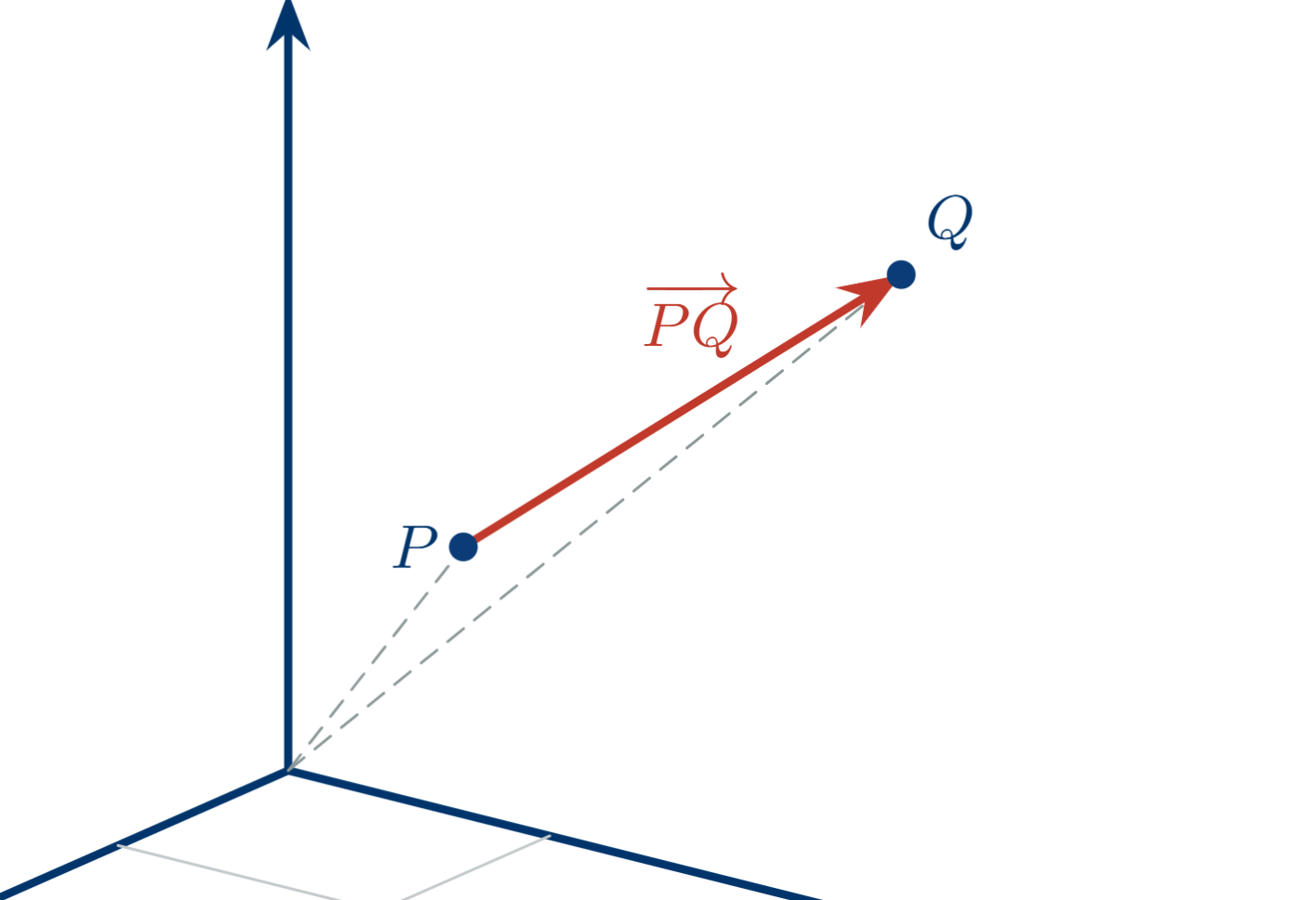
Let's identify $v$ with $P$ and $Q$ through the following application:
\[\delta : \mathcal{A} \times \mathcal{A} \longrightarrow V, \quad (P,Q) \longmapsto v = \overrightarrow{PQ}\]Observe that $v$ is unique for each pair and that there are a few properties that $\delta$ satisfies that are released from the axioms of the affine space:
-
$\overrightarrow{PP} = 0_V$, from $A1$ and simple transitivity.
-
Chasles Relation: $\overrightarrow{PQ} + \overrightarrow{QR} = \overrightarrow{PR}$
Let's quickly observe that: $P + \overrightarrow{PQ} = Q \wedge Q + \overrightarrow{QR} = R$
Thus, using $A2$ we get: $R = Q + \overrightarrow{QR} = (P + \overrightarrow{PQ}) + \overrightarrow{QR} = P + (\overrightarrow{PQ} + \overrightarrow{QR})$, thus:
\[P + (\overrightarrow{PQ} + \overrightarrow{QR}) = R \iff \overrightarrow{PQ} + \overrightarrow{QR} = \overrightarrow{PR}\] -
$\overrightarrow{QP} = -\overrightarrow{PQ}$. This result is immediate from above: $0_V = \overrightarrow{PP} = \overrightarrow{PQ} + \overrightarrow{QP} \iff \overrightarrow{QP} = -\overrightarrow{PQ}$
In this context, we say that the pair $(P,Q)$ or simply $\overrightarrow{PQ}$ is a "bound arrow", with its base in $P$ and its end in $Q$. We formalize this idea applying the $\delta$ construction.
A bound arrow is a pair $(P,v) \in \mathcal{A} \times V$ often related as $(P,\overrightarrow{PQ})$ and interchangeable with $(P,Q)$ since two elements define the third.
Let's pull back briefly to the vector space $(K,(\mathcal{A},+_O),·_O)$.
Let's observe that having fixed $O$, then we can collapse $\delta: A \times A \to V$ to $\delta_O: \mathcal{A} \to V$, verifying:
\[\delta_O( \ ·) = \delta(O, \ · )\]Since the simple transitivity of $+$ imposes a unique displacement from one point to another, fixing one of those points allows us to identify each point on $A$ with a unique "position relative to $O$" vector in $V$.
This means that we can treat each point on $A$ as an arrow from $O$, the identity of the abelian group $(A,+_O)$. In other words, the collection of arrows from an origin has a structure of vector space. This allows us to think of vectors as arrows in a line, plane, space and so on.
3.2.2. Equipolence class: Free vectors.
Let's observe that bound vectors, conceptualized as a displacement, have magnitude, direction and an orientation in the direction. Thus, despite the point of application, two bound vectors are equal if both match these three features.
This leads to the construction of the notion of the free vector as an equivalence class of those bound vectors that share these three features.
3.2.2.1. Appendix: Equivalence Class.
An equivalence class is the set of all elements in a set that we consider "equal" under a certain criterion of equality. The idea is that when we declare certain objects to be interchangeable for our purposes (even if they are not literally the same object), we group together all those that share that quality. That group is the class.
Their importance is structural: equivalence classes are the mechanism that allows us to quotient a set, that is, to create a new set whose points are precisely those packages.
Formally, let $X$ be a non-empty set; an equivalence relation is a binary relation $\sim \ \subseteq X\times X$ satisfying:
- Reflexivity: $\forall x \in X \quad x \sim x$
- Symmetry: $\forall x,y \in X \quad x \sim y \implies y \sim x$
- Transitivity: $\forall x,y,z \quad x \sim y \wedge y \sim z \implies x \sim z$
In this conditions, this equivalence relation defines our criterion to build the equivalence classes $[x]$, formally:
\[[x] :=\ \Set{ y \in X : y \sim x }\]We say that $x$ is the representative of the class. Observe that the following immediate properties are satisfied by the equivalence class:
- $x \in [x] \ \ \forall x \in X$
- $x \sim y \iff [x] = [y]$
-
$\forall x,y \in X \ (x \sim y \oplus x \not \sim y \implies [x] = [y] \oplus [x] \cap [y] = \varnothing)$
This means that two elements of $X$ are either equivalent or not equivalent at all; following the second property, this means that their equivalence classes are disjoint or are the same.
-
$\displaystyle\bigcup_{x \in X} [x] = X$
Lastly, we define the quotient set as:
\[X/\sim := \Set{[x] : x \in X}\]This is the set whose elements are the groups of elements that are qualitatively different according to the $\sim$ criterion.
3.2.2.2. Vector equipolence.
Now, let's say that $X = A \times A$, then we define in $A \times A$ the relation:
\[(P,Q) \sim (P',Q') \iff \overrightarrow{PQ} = \overrightarrow{P'Q'}\]Observe that reflexivity, symmetry and transitivity are immediate from $=$ in $V$. Thus, two bound vectors are equal as long as their displacement is the same in magnitude, direction and orientation despite the application point.
This criterion allows us to define the quotient set:
\[\mathfrak{F}(\mathcal{A}) := (\mathcal{A} \times \mathcal{A})/\sim\]Whose equivalence classes are $[(P,Q)]$. Let's now observe carefully that this structure has a vector space structure.
First, let's fix an origin in $\mathcal{A}$, $O$ and consider the vector space $(K,(\mathcal{A},+_O),·_O)$ and observe that for each equivalence class $[(P,Q)]$, there is some $T \in \mathcal{A} : (O,T) \in [(P,Q)] \iff [(O,T)] = [(P,Q)]$, meaning that we can define:
\[\iota_O : \mathcal{A} \longrightarrow \mathfrak{F}(\mathcal{A}), \qquad P \longmapsto [\,(O,P)\,]\]This function is bijective since $O$ is fixed and we can transport $(+_O, \cdot_O)$ to the quotient set $\mathfrak{F}(\mathcal{A})$ by operating with the canonical representative of each class.
So $(K, (\mathfrak{F}(\mathcal{A}),+_O),·_O)$ is a vector space and this ultimately means that, in an affine space, whenever we treat a vector $v$ we catch the canonical representative of its equivalence class relative to an origin $O$, and work with it as if both were the same vector.
As an example, observe that this matches some known operations with points and vectors. Consider $P,Q \in \mathcal{A}$, we can identify each point with its vector from the origin, $\overrightarrow{OP}, \overrightarrow{OQ}$. Then, by Chasles:
\[\overrightarrow{PQ} = \overrightarrow{PO} +\overrightarrow{OQ} = - \overrightarrow{OP} + \overrightarrow{OQ} \iff \overrightarrow{OP} + \overrightarrow{PQ} = \overrightarrow{OQ}\]Meaning that subtracting $P$ from $Q$ (from any arbitrary point) gives us the displacement from $P$ to $Q$ formalized in $\overrightarrow{PQ}$, and the thing is that we would not work directly with $\overrightarrow{PQ}$ but with the canonical representative of its equivalence class, $\overrightarrow{OT} : \overrightarrow{OT} \sim \overrightarrow{PQ}$
4. Summary.
As a brief summary of the post, we have defined Algebra as a mathematical discipline that deals with the study of the properties of operations. In this context, we developed an algebraic definition of the vector space as an algebraic structure in which a deformation mechanism acts on an abelian group, standardizing the "linear combinations" as the natural operation of this space, understood as independent and field-weighted contributions of elements from the abelian group.
Later, we explored the geometric intuition behind the vector spaces. For that, first we defined the affine space as the object resulting from using a vector space in a simple and transitive way to study a non-empty set. We also saw that the affine space is a "point-uniform" structure and whenever you fix one point as a source of vectors, the affine space acquires a vector space.
Then, we built the concept of "bound vector" as a displacement between two points in the affine space and identified such bound vector with the mathematical object we call "arrow". This way, with an origin fixed, we defined a bijective application that identifies any point with a certain vector from the origin. Thus, the collection of all possible arrows that stem from a point in an affine space has the structure of a vector space and that is the precise visual representation we were searching for.
Ultimately we formalized the bound vector as a "free vector", this being the equivalence class of all the bound vectors that share magnitude, direction and orientation. The set of all free vectors has also a vector space structure which allows us to identify any bound vector on the affine space with its canonical class representative and operate with it as if both were the same vector.
5. Exercises.
5.1. If $F$ is a field, verify that $F^n$ (as defined in Example 1) is a vector space over the field $F$.
Done in $2.3.1.$
5.2. If $V$ is a vector space over the field $F$, verify for all vectors $a_i \in V : i =1,2,3,4$ that:
\[(a_1 +a_2) + (a_3 + a_4) = [a_2 + (a_3 + a_1)] + a_4\]Observe that since $(V,+)$ is an abelian group the exercise is immediate, it is just generalizing the associativity and commutativity for more than two elements.
5.3. If $C$ is the field of complex numbers, which vectors in $C^3$ are linear combinations of $(1, 0, -1), (0, 1, 1), (1, 1, 1)$?
Those resulted in being the composition of any proportional vector of the given ones, formally verifying:
\[v \in \mathbb{C}^3 \mid \exists \alpha, \beta ,\gamma \in \mathbb{C} : v = \alpha(1, 0, -1) +\beta(0, 1, 1)+ \gamma (1, 1, 1)\]Doing the algebraic simplification, we get the family of vectors:
\[\Set{(\alpha + \gamma,\beta + \gamma, \gamma + \beta - \alpha) : \alpha, \beta ,\gamma \in \mathbb{C}} \subset \mathbb{C}^3\]Let's note an interesting observation, if we think about the forms of the vectors in order to extract a restriction, this is, when, for a vector $(x,y,z)$ does not exists $\alpha, \beta, \gamma \in \mathbb{C}:$
\[\begin{cases} x = \alpha + \gamma \\ y = \beta + \gamma \\ z = \gamma + \beta - \alpha \end{cases} \iff \begin{cases} \alpha = x - \gamma \\ \beta = y - \gamma \\ \gamma = z - \beta + \alpha \end{cases}\]Ultimately; $\alpha = y-z, \beta = -x+2y-z, \gamma = x−y+z$, meaning the solution always exists and is unique, so in fact our span set is $\mathbb{C}^3$.
5.4. Let $V$ be the set of all pairs $(x, y) \in \mathbb{R}^2$ of real numbers. Is $(R, V, ·)$ a vector space?. Defined:
\[(x, y) + (x_1,y_1) = (x + x_1, y +y_1)\] \[c(x,y) = (cx,y)\]The addition $+$ is the classic addition operation in $\mathbb{R}^2$ so it is clear that $(V,+) = (\mathbb{R}^2,+)$ is an abelian group. Now, let's take a closer look at the field's action.
Observe that there is something weird; $0 · (x,y) = (0,0) \iff y = 0$ which should not be.
In a proper vector space the ordinary proof of the statement asserts that:
\[0v = (0+0)v = 0v + 0v \iff 0v = 0 \quad \forall v \in V\]And the second equality comes from the axiom $D2$, that states:
\[(\alpha + \beta)v = \alpha v + \beta v \quad \forall \alpha, \beta \in K, v \in V\]But this is not satisfied by the operation:
\[(\alpha + \beta)(x,y) = ((\alpha + \beta)x,y)\] \[\alpha (x,y) + \beta (x,y) = ((\alpha + \beta)x,2y)\]Which is only true when $2y = y \iff y = 0$, so the structure provided does not verify the axioms of the action's field and is not a vector space.
5.5. On $\mathbb{R}^n$, which of the axioms for a vector space are satisfied by $(\mathbb{R}^n, \oplus, · )$ defined:
\[\alpha \oplus \beta = \alpha - \beta\] \[c · \alpha = - c \alpha\]Observe that $\alpha \oplus \beta = \alpha - \beta \neq \beta - \alpha = \beta \oplus \alpha$, so $(\mathbb{R}, \oplus)$ is not an abelian group. Also, the application is not a field action, since the identity does transform the vector; $1\alpha = - \alpha$. Thus, the structure as presented is not a vector space.
5.6. Let $V$ be the set of all complex-valued functions $f$ on the real line such that $\forall t \in \mathbb{R} \quad f(-t) = \overline{f(t)}$, then show that $(V, +,·)$ is a $\mathbb{R}$-vector space with:
\[(f+g)(t) = f(t) + g(t)\] \[(cf)(t)=cf(t)\]Observe that $V := \Set{f \in \mathbb{C}^{\mathbb{R}}\mid f(-t) = \overline{f(t)}}$, thus, let's first check $(V,+)$ is an abelian group:
-
Associativity and Commutativity are immediate from Associativity and Commutativity of addition in $(\mathbb{C},+)$.
Let's check closure: observe that
\[f,g \in V \implies (f+g)(-t) = f(-t) + g(-t) = \overline{f(t)}+\overline{g(t)} = \overline{f(t)+g(t)}= \overline{(f+g)(t)}\]Let's think about the identity element. We have to demonstrate the existence of some element $i \in V$ such that
\[(i+f)=(f+i)=f \quad \forall f \in V\]Let's consider $i \in \mathbb{C}^{\mathbb{R}}: i(t) = 0 \quad \forall t \in \mathbb{R}$, note in first place that $0 = \overline{0} \implies i \in V$, and it satisfies:
\[(i+f)(t)=i(t) + f(t)=f(t)+i(t) = f(t) \quad \forall f \in V\]Lastly, consider some $f \in V$, we have to think in some $-f \in V: (f+-f)=(-f + f)=i$, or, what is the same: $(f+-f)(t) = (-f +f)(t) = 0$.
Let's consider $-f \in \mathbb{C}^{\mathbb{R}}: -f(t) = -(f(t))$, observe that:
\[-f(-t) = -(f(-t))=-(\overline{f(t)}) = \overline{-f(t)} \implies -f \in V\]Then, $(V,+)$ is an abelian group.
Let's check now that $·:\mathbb{R} \times V \to V$ is a field's action:
- Identity; Taking $1 \in \mathbb{R}$, is immediate.
- Associativity: Immediate from associativity in $(\mathbb{R}\setminus\Set{0}, ·)$.
- Compatibility in $V$; Immediate from compatibility in $\mathbb{C}$
- Compatibility in $\mathbb{R}$; Immediate from compatibility in $\mathbb{C}$
Thus, $(\mathbb{R},(V,+),·)$ is a vector space.
As an example of a function in $V$ not real-valued is $f(t) = it$.
5.7. Take the following operations in $\mathbb{R}^2$. Is $(\mathbb{R},(\mathbb{R}^2,+),·)$ a vector space?
\[(a,b) + (c,d) = (a+c,0)\] \[c(a,b) = (ca,0)\]Observe that there is no identity in $(\mathbb{R}^2,+)$ so it is not an abelian group