Modeling & ComputationModelado y Computación
Introduction to Machine Learning.
Introduction to ML. Gradient Descent.
0. Index.
- Machine Learning
- Formal Framing
- Learning Algorithm
- 3.1. Mathematical Prerequisites
- 3.1.1. Functions of Several Variables
- 3.1.2. Partial Derivatives
- 3.1.3. Directional Derivatives
- 3.1.4. Gradient
- 3.1.5. Taylor Expansions
- 3.2. Formal Development
- 3.2.1. Hypothesis Sets
- 3.2.2. Measuring the Error: Cost Function
- 3.3. Gradient Descent Algorithm
- 3.3.1. Optimization. Classical Approach
- 3.3.2. Optimization. Iterative Approach
- 3.3.3. Explaining the Algorithm
- 3.3.4. Descent Mechanism
- 3.1. Mathematical Prerequisites
-
- Summary
1. Machine Learning.
In conventional programming, explicit rules are taught to programs in order to establish solid logic predicates about constraints or bifurcations over the execution flow of the program.
Machine Learning is a family of algorithms that learn patterns from data instead of following explicitly programmed rules. In other terms, Machine Learning is a field of study that gives computers the ability to learn without being explicitly programmed.
2. Formal Framing.
Let's understand what "learning from data" actually mathematically means; the objective is to find a function that captures the regularity of an observed phenomenon that produces data in order to make predictions on new, unseen inputs of the same nature.
Formally, we have the following pieces:
-
An input space, the set of all possible inputs. For instance $\mathcal{X} = \mathbb{R}^n$, thus each input $x$ is a vector of $n$ features.
-
An output space $\mathcal{Y}$, which is the set of all possible outputs. This depends on what is being modeled; in classification problems the output set can be a finite subset of the natural numbers which are the clusters, $\mathcal{Y} = [n]$; for regression, which wants to predict a continuous value, it is $\mathcal{Y} = \mathbb{R}$.
-
The target function, the ideal mapping $\mathcal{X} \to \mathcal{Y}$ that relates each input $x \in \mathcal{X}$ to the desired output $y \in \mathcal{Y}$ which is abstracted in the application $f : \mathcal{X} \to \mathcal{Y}$ and remains unknown. This deterministic presentation is purely pedagogic and more complex in reality, the precise form would be to say that the data pairs arise from an unknown joint probability distribution $P$ over $\mathcal{X} \times \mathcal{Y}$.
-
The training set; a finite subset $\mathcal{D} \subset \mathcal{X} \times \mathcal{Y}$ defined as $\mathcal{D} := \Set{(x_i,y_i)}_{i=1}^m : y_i = f(x_i)$
The goal of ML is to use $\mathcal{D}$ to find a mapping $g_{\mathcal{D}}:\mathcal{X} \to \mathcal{Y} : g_\mathcal{D} \approx f$. Observe that $g_\mathcal{D}$, by definition, allows us to make predictions along all the $\mathcal{X} \times \mathcal{Y}$ space, this is, not only for the inputs from $\mathcal{D}_\mathcal{X}$ but for any $x \in \mathcal{X}$.
We don't search across all possible functions $f: \mathcal{X} \to \mathcal{Y}$; that set is unimaginably large and the problem would be ill-defined. Instead, we choose a hypothesis set; $\mathcal{H}$, which is a restricted family of candidate functions. A learning algorithm selects one of the candidates of $\mathcal{H}$ as $g_\mathcal{D}$.
For example, the linear regression learning model is a supervised learning model (we will see what this is later) in which we assume that $\mathcal{H}$ is the set of all the affine transformations $\mathbb{R}^n \to \mathbb{R}$.
3. Learning Algorithm.
As we set in the previous section, we need to develop a mechanism that allows us to select the best candidate from a family of applications $\mathcal{H}$ that maps correctly - matching our needs - the input $\mathcal{X}$ with the outputs $\mathcal{Y}$ using only the training set $\mathcal{D} \subset \mathcal{X} \times \mathcal{Y}$ established before as a reference. Overall, this selection is based on the question of which $h \in \mathcal{H}$ minimizes as much as possible the noise or incorrectness in the mapping $\mathcal{X} \to \mathcal{Y}$ done by $h$.
The learning algorithm is the procedure that actually performs this search. In practice, for the vast majority of modern ML, this reduces to a continuous optimization problem: minimize a real-valued function (the loss function; the one that measures the error over the predictions) over a space of parameters.
3.1. Mathematical Prerequisites.
3.1.1. Functions of Several Variables.
A function of $n$ real variables is a map:
\[f : S \to \mathbb{R} , \quad S \subset \mathbb{R}^{n}\]Where:
- $S$ is the evaluation domain
- $\mathbb{R}$ is the codomain
Then, the input is a vector with $n$ coordinates $x := (x_1,\cdots,x_n) \in \mathbb{R}^n$ and the image of $x$ through $f, f(x) \in \mathbb{R}$ is a real scalar.
It is worth visualizing that for $n = 2$, the plot of $f(x,y)$ on $x,y$ is a surface given by the parameters $(x,y,f(x,y)) \in \mathbb{R}^3$, $f(x,y)$ is the height in the plane formed by the coordinates $(x,y) \in \mathbb{R}^2$. Now, if $n >3$ the geometric visualization breaks, while the math holds in the sense that $f(x)$ is the height at each point of $\mathbb{R}^n$.
In ML, the models we work with depend on a vector of adjustable parameters $\boldsymbol{\theta} \in \mathbb{R}^p$ where $p$ depends on the model architecture and can range from a handful to billions. Training these models requires understanding how each parameter affects the output, which demands the machinery of functions of several variables.
3.1.2. Partial Derivatives.
Let $ f: S \to \mathbb{R}, \quad S \subseteq \mathbb{R}^n$ be now a multivariable function; let's choose a point $\mathbf{a}:=(a_1,\ldots,a_n) \in S$.
Then, we define the partial derivative of $f$ respect to $x_i$ at $\mathbf{a}$ as (provided this limit exists):
\[\frac{\partial f}{\partial x_i}(\mathbf{a}) = \lim_{t \to 0} \frac{f(\mathbf{a} + te_i) - f(\mathbf{a})}{t} =\] \[= \lim_{t \to 0} \frac{f(a_1,\ldots,a_{i-1}, a_i + t, a_{i+1},\ldots,a_n) - f(a_1,\ldots,a_n)}{t}\]Where $e_i$ is the $i$-th standard basis vector.
It is important to note the partial derivative is just the extension of the single-variable derivative applied to a multivariable function on one single feature $x_i$, meaning that the scalar $t \in \mathbb{R}$ perturbs only the $i$-th coordinate (literally an ordinary single-variable derivative applied to a function where all variables except one have been frozen to constants).
A formal treatment is to define $g_i: \mathbb{R} \to \mathbb{R}$ from $f$ by:
\[g_i(t) = f(a_1,\ldots,a_{i-1},t,a_{i+1},\ldots,a_n)\]Then, the partial derivative acquires another representation:
\[\frac{\partial f}{\partial x_i}(\mathbf{a}) = g'_i(a_i) = \lim_{h \to 0} \frac{g_i(a_i + h)-g_i(a_i)}{h}\]A simple exchange $g_i \leftrightarrow f$ returns to us the original definition, but this shape gives a more intuitive approach since we can understand the partial derivative from our understanding of the single-derivative concept with which we are already familiar.
The formula above tells us that the partial derivative tells us how $f$ changes under a minimal (differential) change of the $i$-th feature, maintaining the rest of the variables as constants.
Geometric Interpretation
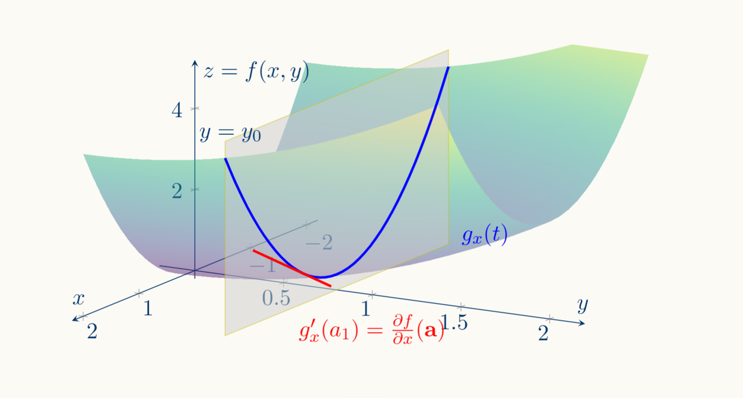
Let's take the case $n=2$, the graph of $f : \mathbb{R}^2 \to \mathbb{R}$ is a surface on $\mathbb{R}^3$; $(x,y,f(x,y)) \in \mathbb{R}^3$.
In this context, the function $g_x:\mathbb{R} \to \mathbb{R} \ \vert \ g_x(t) := f(t,y_0)$ describes the curve of $f$ in the plane $(x,f(x,y_0)) \in \mathbb{R}^2$ which is the section given by the plane $y=y_0$ on the surface $(x,y,f(x,y)) \in \mathbb{R}^3$
This way, $\frac{\partial f}{\partial x}(a) = g_x'(a)$ is the slope of the tangent line to that curve at the point $(a_1,a_2,f(a_1,a_2))$. The geometric interpretation of the single-variable derivative carries over directly: you are just reading the slope on a specific slice of the surface:
In general, the graph of $f:\mathbb{R}^n \to \mathbb{R}$ is a hypersurface in $\mathbb{R}^{n+1}$, freezing all coordinates except $x_i$ defines a line in $\mathbb{R}^n$, the image of that line under the graph map $x \mapsto (x, f(x))$ is a curve on the hypersurface, and $D_if(\mathbf{a})$ is the slope of the tangent line to that curve.
In summary, partial derivatives measure how $f$ changes when we adjust one parameter while keeping all others fixed. This is needed to form the gradient which basically is a vector that tells us the movement tendency of $f$ at a point in $\mathbb{R}^n$
3.1.3. Directional Derivatives.
Definition
Let's barely introduce what the directional derivative is.
Observe that the partial derivatives we've just presented above measure the change ratio along the coordinate that isn't frozen. In the example we proposed, the curve is the intersection of the surface with the plane $y = y_0$, thus, the partial derivative explore how $f$ changes along the $x$ coordinate axis.
Thus, partial derivatives measure rates of change along coordinate axes, now directional derivatives introduce how to measure this change along virtually any direction. The directional derivative generalizes partial derivatives to arbitrary directions.
Let $E \subseteq \mathbb{R}^n$ be open, and let $f: E \to \mathbb{R}$ be differentiable at $\mathbf{a} \in E$. Then, we define the directional derivative of $f$ at $\mathbf{a}$ in the direction of $\mathbf{u}$:
\[D_{\mathbf{u}} f(\mathbf{a}) = \lim_{t \to 0} \frac{f(\mathbf{a}+t\mathbf{u}) - f(\mathbf{a})}{t}\]Where $\mathbf{u}$ is a unit vector, a vector with direction but without disturbing magnitude (this is, so to speak, the modulus is $\vert \vert u \vert \vert = 1$, thus it does not disturb the magnitude of any other vector). Let's take a closer look.
If is $\mathbf{u} := (u_1,\ldots,u_n) \in \mathbb{R}^n : \vert \vert u \vert \vert = 1$, then $t\mathbf{u}$ is a scalar multiplication on $\mathbf{u}$,
\[t\mathbf{u}:=(tu_1,\ldots,tu_n) \implies \mathbf{a} + t\mathbf{u} := (a_1 +tu_1,\ldots, a_n+tu_n)\]Every coordinate gets perturbed simultaneously, each by the amount $tu_i$. The vector $\mathbf{u}$ controls the direction of the perturbation, and the scalar $t$ controls how far you go in that direction.
Geometric Interpretation
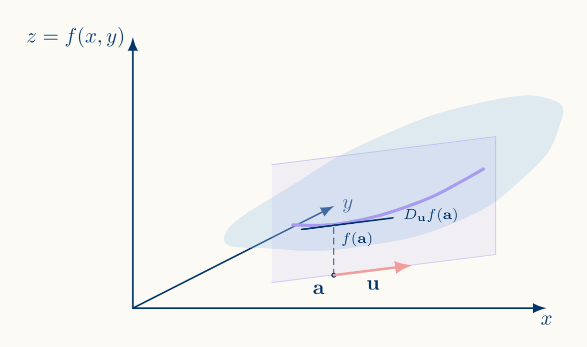
This means that the geometric interpretation remains the same, but now the plane contains the line passing through the point $\mathbf{a}$ with the direction of the unit vector $\mathbf{u}$. This plane is no longer parallel to any coordinate axis but extends in the direction of $\mathbf{u}$.
As a visual example, for $f:\mathbb{R}^2 \to \mathbb{R}$ the intersection of this plane and the surface gives us a curve containing $(\mathbf{a},f(\mathbf{a}))$, then $D_uf(\mathbf{a})$ is the slope of the tangent line to the curve at $\mathbf{a}$
3.1.4. Gradient.
Definition
Consider now $f: S \subset \mathbb{R}^n \to \mathbb{R}$ and a point $\mathbf{a} \in \mathbb{R}^n: \exists \partial_if(\mathbf{a}) \ \forall i \in [n]$. We define as the gradient of $f$ at $\mathbf{a}$ to the vector:
\[\nabla f(\mathbf{a}) := \begin{pmatrix} \frac{\partial f}{\partial x_1}(\mathbf{a})\\ \vdots\\ \frac{\partial f}{\partial x_n}(\mathbf{a}) \end{pmatrix} \in \mathbb{R}^n\]Observe that the gradient lives in the domain of $f$, $\mathbb{R}^n$, not in the hypersurface $\mathbb{R}^{n+1}$.
Geometric Interpretation
Now, lets recover the directional derivative definition:
\[D_{\mathbf{u}} f(\mathbf{a}) = \lim_{t \to 0} \frac{f(\mathbf{a}+t\mathbf{u}) - f(\mathbf{a})}{t}\]Observe that, by the chain rule (assuming $f$ is differenciable at $\mathbf{a}$), we have the following result:
\[D_\mathbf{u} f(\mathbf{a}) = \nabla f(\mathbf{a})\ · \mathbf{u}\]Observe that $\nabla f(\mathbf{a})\ · \mathbf{u} = \Vert \nabla f(\mathbf{a}) \Vert \Vert \mathbf{u} \Vert \cos\theta$, which means that $D_\mathbf{u} f(\mathbf{a})$ is maximum when $\mathbf{u}$ and $\nabla f(\mathbf{a})$ have the same direction $\cos\theta = 1 \implies \theta = 0 \pmod {2\pi}$.
Thus, in general, the gradient $\nabla f(\mathbf{a})$ always points towards the direction in which the slope of the tangent line to the curve on the surface ($D_\mathbf{u}f(\mathbf{a})$) is maximum, this is what we call the steepest ascent direction.
Then $-\nabla f(\mathbf{a})$ always points towards the direction in which the slope is minimum, the steepest descent direction. This geometric property justifies the gradient descent algorithm we will see later.
3.1.5. Taylor Expansions.
Taylor formulas solve a fundamental problem; locally approximating a complicated function by a polynomial, which is the most tractable object in analysis.
The result asserts that, if a function is smooth enough (differentiable several times) at a point $\mathbf{a}$, then its behavior near $\mathbf{a}$ is captured, with controlled error, by a polynomial whose coefficients are the successive derivatives at $\mathbf{a}$.
Taylor Theorem (with Lagrange Remainder)
Let $f: [a, b] \to \mathbb{R}$ with $f^{(n)}$ continuous on $[a,b]$ and $f^{(n+1)}$ existing on $(a,b)$. Then:
\[\forall x \in (a,b] \ \ \exists c \in (a,x): f(x) = \sum_{k=0}^{n} \frac{f^{(k)}(a)}{k!}(x-a)^k + \frac{f^{(n+1)}(c)}{(n+1)!}(x-a)^{n+1}\]Observe that, despite being an exact equality (the function is its Taylor polynomial plus an error term with an explicit form), the $c$ term in the Lagrange remainder remains unknown.
Nevertheless, the result is powerful since we are predicting information about $f$ in an interval using only local information at a single point.
Expansion: Peano's Remainder
There is another form of the remainder that is weaker but often more useful for optimization arguments. Under the same hypothesis:
\[f(x) = \sum_{k=0}^{n} \frac{f^{(k)}(a)}{k!}(x-a)^k + o(|x-a|^n)\]where $o(|x-a|^n)$ means that $\displaystyle\frac{R_n(x)}{|x-a|^n} \to 0$ as $x \to a$ and at some point where, $x$ becomes close enough to $a$, the error factor becomes negligible.
Definition: Taylor's multivariate extension and Geometric Intuition
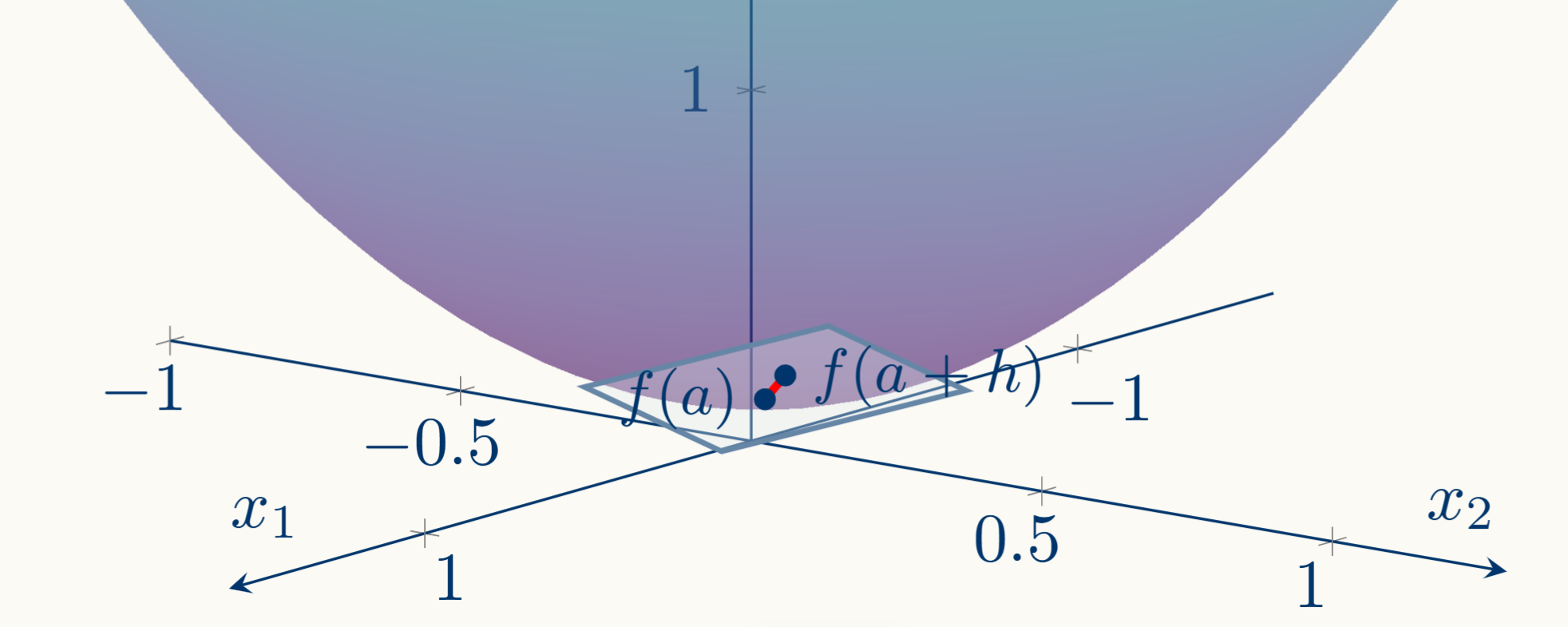
For $f: \mathbb{R}^d \to \mathbb{R}$ differentiable on $\mathbf{a}$, the first-order Taylor expansion around a point $\mathbf{a}$ evaluated at $\mathbf{a} + \mathbf{h}$ is:
\[f(\mathbf{a} + \mathbf{h}) = f(\mathbf{a}) + \nabla f(\mathbf{a})^\top \mathbf{h} + o( \Vert \mathbf{h} \Vert)\]Where $ o( \Vert \mathbf{h} \Vert)\to 0$ as $ \alpha \to 0$.
At $\mathbf{a}$, the graph of $f$ (a surface in $\mathbb{R}^{p+1}$) has a tangent hyperplane. The Taylor expansion says: the function value at a nearby point equals the tangent hyperplane's value at that point, plus an error that becomes negligible as you zoom in.
3.2. Formal Development.
3.2.1. Hypothesis Sets.
As we said before, we don't search for a hypothesis $h$ in the abstract; we first form a family of candidates $\mathcal{H}$. This is parameterized by a vector of real numbers $\theta \in \mathbb{R}^p$:
\[\mathcal{H} := \Set{h_\theta : \mathcal{X} \to \mathcal{Y} \ \vert \ \theta \in \Theta}\]Where,
-
$\theta = (\theta_1, \ldots, \theta_p) \in \mathbb{R}^p$.
Is the parameter vector. Each specific $\theta$ picks out one specific hypothesis $h_{\theta} \in \mathcal{H}$.
-
$p \in \mathbb{N}$, is the number of parameters (in modern deep learning, $p$ can be in the billions).
-
$\Theta \subseteq \mathbb{R}^p$ is the parameter space over all $\mathbb{R}^p$
Linear Model
As a brief example, let's take a look at the linear model, which, as we said before, is the assumption that $h$ is an affine transformation. Remember that an affine transformation is a linear transformation $y=mx$ plus a translation $b$, taking the form of the line: $y_{m,b} := b + mx$, then in our parameterized function:
\[h_\theta(\mathbf{x}) := \theta_0 + \boldsymbol{\theta^{\top}} · \ \mathbf{x} = \theta_0 + \sum_{i=1}^{p-1} \theta_i x_i\]Where $\theta_0$ is the bias and $\theta_i \ \forall i \in [p-1]$ is the parameter of the $i$-th feature $x_i$. Observe that each $\theta$ gives us a different linear function.
3.2.2. Measuring the error: Cost function.
It is reasonable to ask, for a certain $\theta$, how far the prediction is from the real, labeled, output. Formally; for a pair $(x,y) \in \mathcal{X} \times \mathcal{Y}$, how wrong is the prediction $h_\theta(x)$, let's first formalize the notion of 'wrong' in mathematical terms.
Loss Function
Let's define:
\[L : \mathcal{Y} \times \mathcal{Y} \to \mathbb{R}_{\geq 0}\]$L(y,h_\theta(x))$ takes the true value $y$ and the predicted value $h_\theta(x)$ and returns a non-negative real number: the penalty for that single prediction. The larger $L(y,h_\theta(x))$, the worse the prediction.
The loss function is a design choice; different losses encode different priorities about what kinds of errors matter based on the space in which the output set is defined. For example, applied to the linear regression model, the output space is $\mathbb{R}$ which is a metric space, thus, the loss function adopts the form of the squared loss; penalizes errors proportionally to the square of the deviation; large errors are punished disproportionately.
\[L(y,h_\theta(x)) := (y - h_\theta(x))^2\]But note that $L$ only measures error at a single point. A model doesn't predict one point; it predicts across the entire input space. We need to aggregate.
True Risk
The natural next question: how wrong is $h_{\boldsymbol{\theta}}$ across all the input space.
Ideally, we would measure the expected loss over the entire data-generating process. The data comes from some unknown probability distribution $P$ over $\mathcal{X} \times \mathcal{Y}$; this unknown probability pattern associates inputs to outputs in what we call the phenomenon data. Think for example of the height and the age of a person; it is the formal way of saying "nature produces input-output pairs according to some pattern".
The population risk, also called true risk, of a hypothesis $h$ is:
\[R(h) = \mathbb{E}_{(x,y) \sim P}\big[L(y, h(x))\big]\]This is a sum (or integral, in the continuous case) over all possible pairs $(x, y) \in \mathcal{X} \times \mathcal{Y}$, each weighted by its probability under $P$. It captures the average error of $h$ across the entire distribution, including inputs you'll never see in your training set.
This the object we truly want to minimize. It captures how well $h$ performs on all data, including data we haven't seen.
However, the fundamental problem is we cannot compute $R(h)$ since it is based on $P$ and the distribution $P$ is unknown (if we knew it, we would know $f$, and there would be no learning problem). $R(h)$ is a theoretical ideal, not a computable quantity.
Empirical Risk
A reasonable approximation to the true risk (based on $P$) is the empirical risk based on a dataset we have access to: $\mathcal{D}$. The empirical risk of $h$ on $\mathcal{D}$ is:
\[\hat{R}_{\mathcal{D}}(h) = \frac{1}{m}\sum_{i=1}^{m} L\big(y^{(i)}, h(x^{(i)})\big)\]Observe that, as a discrete, finite sample, the expected value $\mathbb{E}_{(x,y) \sim P}$ converges to a sum. Each training example gets weight as $\frac{1}{m}$, we treat them all equally because we don't know $P$ so we assume that they are all probably equal.
This is the average loss computed on the $m$ training examples a quantity we can compute, because we know every $(x^{(i)}, y^{(i)}) \in \mathcal{X} \times \mathcal{Y}$ and we can evaluate $h(x^{(i)})$.
The empirical risk is a finite-sample estimate of the true risk. Under reasonable conditions, the law of large numbers guarantees that as $m \to \infty \implies \hat{R}_{\mathcal{D}}(h) \to R(h)$.
At this point, we would think that an acceptable strategy to choose $h_\theta$ is to choose an $h$ that minimizes $\hat{R}_{\mathcal{D}}$, which is what we call the Empirical Risk Minimization:
\[h^* = \arg\min_{h \in \mathcal{H}} \hat{R}_{\mathcal{D}}(h)\]Let's observe that $\min_{a\in A}f(a)$ is the minimum value $f$ returns in a subset of his evaluation domain, then $\arg\min_{a\in A}f(a)$ is the input (the argument) that produces that minimum value.
This is conceptually clean, but still abstract because we're minimizing over a set of functions $\mathcal{H}$. To make this into an actual algorithm we can run on a computer, we need one more step.
The Cost Function
Since every $h \in \mathcal{H}$ is indexed by a parameter vector $\theta \in \mathbb{R}^p$, the empirical risk becomes a function of $\theta$:
\[J: \mathbb{R}^p \to \mathbb{R}, \quad J(\theta) := \hat{R}_{\mathcal{D}}(h_{\theta}) = \frac{1}{m}\sum_{i=1}^{m} L\big(y_i,\; h_{\theta}(x_i)\big)\]This function measures the global error in the training set between the prediction and the labeled data; it is the cost function (also called objective function). Observe carefully that having a provided training set $\mathcal{D}$, and an appropriate loss function $L$, the last free variable is $\theta$.
The learning problem has become to find:
\[\boldsymbol{\theta}^* = \arg\min_{\boldsymbol{\theta} \in \Theta} J(\boldsymbol{\theta})\]Find the point in $\mathbb{R}^p$ where $J$ attains its minimum. This is a standard optimization problem where all the math presented before applies.
Each step is forced by the limitations of the previous one: $L$ only measures one point, so we average to get $R$; $R$ is not computable, so we approximate with $\hat{R}_{\mathcal{D}}$;$\hat{R}_{\mathcal{D}}$ is still abstract over $\mathcal{H}$, so we parameterize to get $J(\theta)$, which is a concrete function in $\mathbb{R}^p$ that we can differentiate and minimize with gradient descent.
3.3. Gradient Descent Algorithm.
We arrived at a concrete problem: we modeled a function $J$ that measures the error of the prediction function $h_\theta$ over the training set $\mathcal{D} \subset \mathcal{X} \times \mathcal{Y}$ that depends on the parameter $\theta$. The objective is to find the $\theta$ that minimizes the error, this is, that minimizes the $J$ output.
3.3.1. Optimization. Classical Approach.
An optimization problem is, in its most general form, the task of finding the input to a function that produces the smallest (or largest) output value. For our purposes, we want to find the value for $\theta \in \mathbb{R}^p$ that minimizes the $J$ output. Again:
\[\theta^* = \arg\min_{\theta \in \Theta}J(\theta)\]That's it, we have a real-valued function of several variables and we want the point where it attains its minimum. This is an extremely old and central problem in mathematics. The ML learning problem becomes an optimization problem the moment we parameterize $\mathcal{H}$ in terms of $\theta$ and define $J(\theta)$; finding the best hypothesis reduces to finding the lowest point of a surface in $\mathbb{R}^p$.
Classically, for example, in a one-variable function context, we would leverage the geometric interpretation of the derivative of a continuous function at a point (with which we are already familiar from the prerequisite section) as the slope of the tangent line to the function and attempt to calculate the point in which that slope is horizontal, this is, zero: $\theta_0 \in \mathbb{R} : J'(\theta_0) = 0$
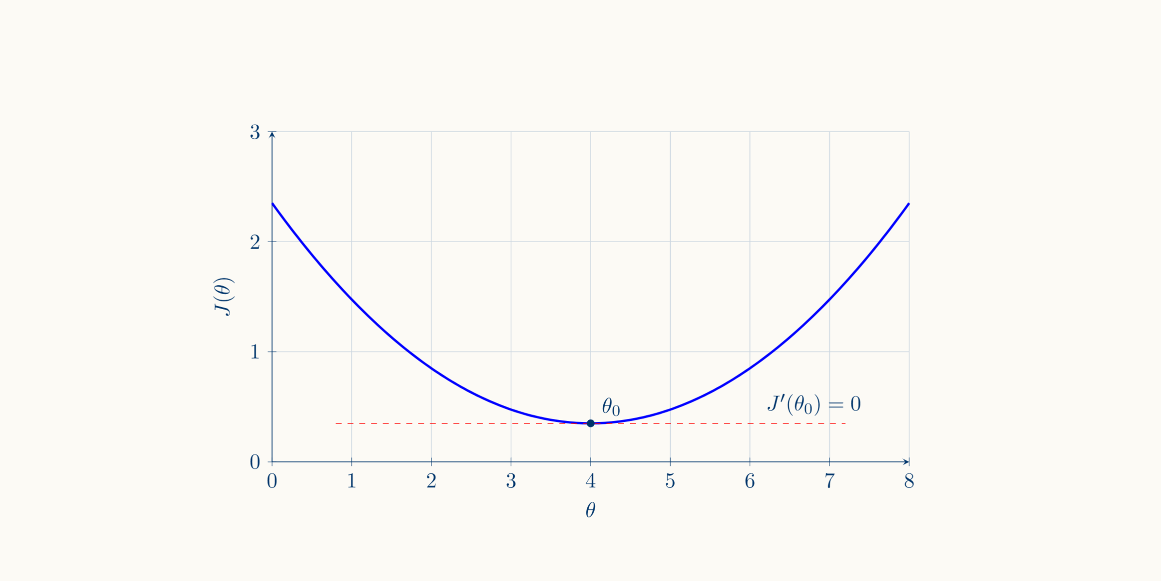
This is a first approach and necessary condition (although not sufficient since other points like local maxima satisfy it). In multiple variables, as far as we know, the most similar tool we have is the gradient which we already saw points towards the steepest ascent direction. This property is furnished from each partial derivative which have a similar geometric interpretation as the derivative in the example above. In a local minimum, the slope of the tangent line to the curve formed by the surface of the function and each plane $x_i=x_0$ is $0$, thus, $\nabla J(\theta_0) = 0$ and points to no direction.
Successful Example. Linear equations.
Let's take the linear regression model presented before, the hypothesis $h_\theta(\mathbf{x}) = \theta_0 + \boldsymbol{\theta}^\top \mathbf{x}$, and let's suppose that our loss function is the squared loss $L(y,h_\theta(\mathbf{x})) = (y - h_\theta(\mathbf{x}))^2$. Then, the cost function would be:
\[J(\theta):=\frac{1}{m} \sum_{i=1}^m L(y,h_\theta(\mathbf{x})) = \frac{1}{m} \sum_{i=1}^m (y^{(i)} - \theta_0 - \boldsymbol{\theta}^\top \mathbf{x}^{(i)})^2\]And the gradient is:
\[\nabla J(\theta) := \left( \frac{\partial J}{\partial \theta_t}(\theta)_{t1} \right)_{t \in [p]} \in \mathbb{R}^p :\quad \frac{\partial J}{\partial \theta_t}(\theta) := -\frac{2}{m}\sum_{i=1}^m (y^{(i)} - \theta_0 - \boldsymbol{\theta}^\top \mathbf{x}^{(i)})x_t^{(i)}\]Observe that $\nabla J = \mathbf{0}$ becomes a system of $p$ linear equations in $p$ unknowns. The solution tells us exactly the point because linear algebra gives us a well-known algebraic method to solve linear systems of equations.
Unsuccessful example. Non-linear equations.
Let's consider now a simple neural network. The relations are multiple and $h_\theta$ is not linear in $\theta$, as an example:
\[h_{\boldsymbol{\theta}}(\mathbf{x}) = \sigma\!\Big(\sum_{k} w_k^{(2)}\; \sigma\!\Big(\sum_{j} w_{kj}^{(1)} x_j + b_k^{(1)}\Big) + b^{(2)}\Big)\]where $\sigma$ is a nonlinear function.
When you compute $\nabla J$ and set it to $0$, you get a system of $p$ equations in $p$ unknowns where the equations involve more than additions and scaling of the unknowns (products of parameters, exponentials of parameters, compositions of nonlinear functions of parameters, etc).
This is a nonlinear system of equations, and there is no general algebraic method for solving systems of nonlinear equations. Also, even if a solution is found $J$ typically has multiple critical points, many local minima, local maxima, and saddle points (modern models handle millions or billions of parameters). The equation $\nabla J = 0$ synthesizes the constraints imposed over all the critical points; solving it gives you all those points and distinguishing among them is itself a hard problem.
Thus, as a summary, the problems of the direct approach are Algebraic Intractability, Multiple critical points and Scale.
3.3.2. Optimization. Iterative Approach.
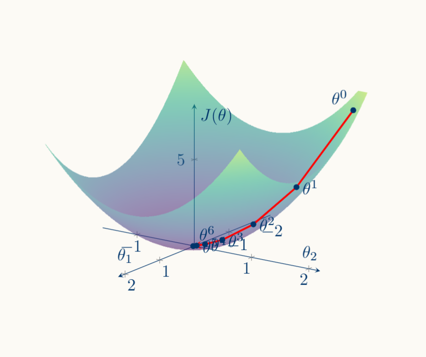
Since we can't find $\theta^\ast$ in one shot, we settle for an iterative strategy: start at some $\theta^{(0)}$, and apply a rule that produces a finite $k$ steps sequence $\theta^{(0)}, \theta^{(1)}, \theta^{(2)}, \dots, \theta^{(k)}:J(\theta^{(t+1)})<J(\theta^{(t)}) $, this is that $J$ decreases at each step.
We may never reach $\theta^* \in \Theta : \nabla J(\theta^*)=0$ exactly, but we can get arbitrarily close which in practice, is perfectly adequate. The core insight is we trade an unsolvable global equation for a sequence of cheap local computations.
3.3.3. Explaining the algorithm.
Until now we have presented the problem and developed a motivation about the need for an iterative method.
Let's develop the brief explanation presented before about the Gradient Descent Algorithm. We said that we need a finite sequence $\theta^{(0)}, \theta^{(1)}, \ldots$ such that the image of $\theta$ through $J$ gets smaller in each step. Thus, given a position $\theta^{(t)}$ we need a procedure to calculate some $\theta^{(t+1)}:J(\theta^{(t+1)}) < J(\theta^{(t)})$ here is when we retrieve the Gradient concept presented on section $1.3.1.4$
We already explained that, being $f :S \subset \mathbb{R}^n \to \mathbb{R}$, the gradient $\nabla f(\mathbf{a}) \in \mathbb{R}^n$ is a vector that points towards the steepest ascent, meaning that it provides information about the behaviour of $f$ in an infinitesimal environment of $\mathbf{a}$ aiming towards the direction that maximizes $f$'s growth (it doesn't aim at the global maximum nor the local maximum).
We remember that if $\nabla f$ points to the steepest ascent, then $-\nabla f$ points to the steepest descent. Thus, recovering our cost function $J$, for a generic $\theta^{(t)}$ the next $\theta^{(t+1)}$ can be calculated according to the gradient:
\[\theta^{(t+1)}:= \theta^{(t)} - \alpha \nabla J(\theta^{(t)}): \alpha \in \mathbb{R}_{>0}\]Where $\alpha > 0$ is called the learning rate and determines how wide is the step between $\theta^{(t)}$ and $\theta^{(t+1)}$.
If $\theta \in \mathbb{R}^p$, then, a component-wise reformulation would be:
\[\theta_j^{(t+1)} = \theta_j^{(t)} - \alpha \, \frac{\partial J}{\partial \theta_j}(\boldsymbol{\theta}^{(t)}), \quad \forall \, j \in [p]\]Each parameter $\theta_j$ is adjusted independently by the partial derivative of $J$ with respect to that parameter, scaled by $\alpha$.
3.3.4. Descent Mechanism.
The algorithm, as we just saw, is pretty simple in theory. We only need to adjust the learning rate parameter and, iteratively, we can get as close as we want to a local minimum.
Let's explore now why this descent is mathematically guaranteed. As a brief explanation, Gradient Descent works since Taylor expansions let you "see beyond" each current point when the next point is close enough. Taylor allows reconstructing $J$'s behavior in a neighborhood around $\theta^{(t)}$, making it possible to see clearly that the next point $J(\theta^{(t+1)})$ is smaller than the current one $J(\theta^{(t)})$.
Consider again the cost function we built above such $J : \mathbb{R}^p \to \mathbb{R}$
\[J(\theta):=\frac{1}{m} \sum_{i=1}^m L(y,h_\theta(\mathbf{x}))\]For our purposes, we will assume that $J$ is differentiable; this assumption holds for the models we've seen so far, although there are activation functions used in practice that are not differentiable everywhere.
Let's take, if $\theta^{(t+1)}:= \theta^{(t)} - \alpha \nabla J(\theta^{(t)}): \alpha \in \mathbb{R}_{>0} \implies \mathbf{h} = - \alpha \nabla J(\theta^{(t)})$, then the first-order expansion:
\[J(\boldsymbol{\theta}^{(t+1)}) = J(\boldsymbol{\theta}^{(t)}) + \nabla J(\boldsymbol{\theta}^{(t)}) \cdot \big(-\alpha\,\nabla J(\boldsymbol{\theta}^{(t)})\big) + o\!\left(\left \Vert -\alpha\,\nabla J(\boldsymbol{\theta}^{(t)})\right \Vert \right)\]Observe that we can simplify the expression:
-
The linear term:
\[\nabla J(\boldsymbol{\theta}^{(t)}) \cdot \big(-\alpha\,\nabla J(\boldsymbol{\theta}^{(t)})\big) = -\alpha\,\nabla J(\boldsymbol{\theta}^{(t)}) \cdot \nabla J(\boldsymbol{\theta}^{(t)}) = -\alpha\,\left \Vert \nabla J(\boldsymbol{\theta}^{(t)})\right \Vert ^2\]We used the property that $\mathbf{v} \cdot \mathbf{v} = \Vert \mathbf{v} \Vert ^2 \ \ \ \forall \mathbf{v} \in \mathbb{R}^p$
-
The error term:
\[o\!\left(\left \Vert -\alpha\,\nabla J(\boldsymbol{\theta}^{(t)})\right \Vert \right) = o\!\left(\alpha\,\left \Vert \nabla J(\boldsymbol{\theta}^{(t)})\right \Vert \right)\]since $ \Vert -\alpha \mathbf{v} \Vert = \vert \alpha \vert \Vert \mathbf{v} \Vert = \alpha \Vert \mathbf{v} \Vert$ (as $\alpha > 0$).
Then, assembling: \(J(\boldsymbol{\theta}^{(t)}) = J(\boldsymbol{\theta}^{(t+1)}) + \alpha\,\left \Vert \nabla J(\boldsymbol{\theta}^{(t)})\right \Vert ^2 - o\!\left(\alpha\,\left \Vert \nabla J(\boldsymbol{\theta}^{(t)})\right \Vert \right)\)
Observe that $\alpha\, \Vert \nabla J(\boldsymbol{\theta}^{(t)}) \Vert ^2 - o(\alpha\, \Vert \nabla J(\boldsymbol{\theta}^{(t)}) \Vert ) > 0$ since $o(\alpha \Vert \nabla J \Vert )$ goes to zero faster as $\alpha \to 0$ while the first term has the fixed positive coefficient $ \Vert \nabla J \Vert ^2$; thus a small enough learning rate $\alpha > 0$ allows us to assert:
\[J(\boldsymbol{\theta}^{(t)}) > J(\boldsymbol{\theta}^{(t+1)})\]Observe that, in a pragmatic way, the role of the learning rate is crucial; all the theoretical justification spins around the size of $\alpha$. Too large: the steps overshoot the minimum; too small: convergence is extremely slow. The algorithm takes tiny steps and may require an impractical number of iterations.
There is no closed-form formula for the optimal learning rate in general; it is tuned empirically or adapted by more sophisticated algorithms.
4. Summary.
Thus, essentially, Machine Learning is applied maths.