Modeling & ComputationModelado y Computación

Linear Algebra for Machine Learning

Linear Algebra Chapter in MML book.

1. Introduction.

When formalizing intuitive concepts, a common approach is to construct a set of objects (symbols) and a set of rules to manipulate these objects. This is known as an algebra; the study of symbolic manipulation and relation of structures. Essentially, algebra studies what is preserved under operations and mappings.

Linear Algebra is the study of those properties that are preserved under linear transformations (transformations that respect addition and scalar multiplication), these are: vectors spaces.

A vector is an element of a vector space. A vector space is not a bare set; it is a set $S$ equipped with two operations (addition and scalar multiplication over a field $F$) satisfying eight axioms. The definition is purely structural: vectors have no privileged concrete representation. Arrows, tuples, polynomials, and matrices can all be vectors when you define the right operations on them and verify the axioms.

In general, vectors are special objects that can be added together and multiplied by scalars to produce another object of the same kind. From an abstract mathematical viewpoint, any object that satisfies these two properties can be considered a vector. Some examples of such vector objects are geometric vectors, polynomials, tuples of $\mathbb{R}^n$ or matrices.

2. System of Linear Equations.

2.1. Formal definition.

A system of linear equations over a field $F$ is a finite collection of equations of the form:

\[a_{i1}x_1 + a_{i2}x_2 + \cdots + a_{in}x_n = b_i, \qquad i = 1,\ldots,m\]

Where the $a_{ij}, b_i \in F$ are given scalars and $x_1, \ldots, x_n$​ are unknowns. They are basically a set of constraints that points of $F^n$ must satisfy simultaneously.

The solution set is $S = {x \in F^n : Ax = b}$. Three things can happen:

• $S = \varnothing$ (inconsistent)

• $\vert S \vert = 1$ (unique solution)

• $\vert S \vert = \infty$

When $b = 0$ (the homogeneous case), $S$ is always nonempty (it contains $0 \in F^n$) and is in fact a subspace of $F^n$.

2.2. Geometric Interpretation of Systems of Linear Equations.

As an illustrative example of how these systems work as constraints over points, let's talk about the geometric interpretation of a system of linear equations in two variables.

In a system of linear equations with two variables $x1, x2$, each linear equation defines a line on the $x1x2$-plane.

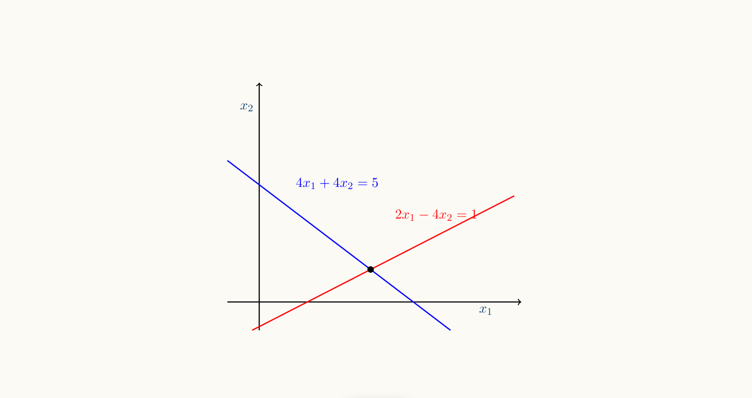
Since a solution to a system of linear equations must satisfy all equations simultaneously, the solution set is the intersection of these lines.

This intersection set can be a line (if $\vert S \vert = \infty$ and the equations describe the same line), a point (if $\vert S \vert = 1$, unique solution), or empty ($S = \varnothing$ , when the lines are parallel).

Similarly, for three variables, each linear equation determines a plane in three-dimensional space. When we intersect these planes, i.e., satisfy all linear equations at the same time, we can obtain a solution set that is a plane, a line, a point or empty (when the planes have no common intersection).

3. Matrices.

For a systematic approach to solving systems of linear equations, we will introduce a useful compact notation. We collect the coefficients $a_{ij}$ into vectors and collect the vectors into matrices. In other words, we write the system from above in the following form:

\[x_1 \begin{bmatrix} a_{11}\\ \vdots\\ a_{m1} \end{bmatrix} + x_2 \begin{bmatrix} a_{12}\\ \vdots\\ a_{m2} \end{bmatrix} + \cdots + x_n \begin{bmatrix} a_{1n}\\ \vdots\\ a_{mn} \end{bmatrix} = \begin{bmatrix} b_1\\ \vdots\\ b_m \end{bmatrix} \iff\] \[\iff \begin{bmatrix} a_{11} & \cdots & a_{1n}\\ \vdots & & \vdots\\ a_{m1} & \cdots & a_{mn} \end{bmatrix} \begin{bmatrix} x_1\\ \vdots\\ x_n \end{bmatrix} = \begin{bmatrix} b_1\\ \vdots\\ b_m \end{bmatrix} \iff A X = Y\]

In this context, we say that $A$ is the coefficient matrix, $X$ is the unknown matrix and $Y$ is the constant matrix.

Matrices play a central role in linear algebra. They can be used to compactly represent systems of linear equations, but they also represent linear functions (linear mappings) as we will see later. Before we discuss some of these interesting topics, let us first define what a matrix is and what kind of operations we can do with matrices.

3.1. Definition and Operations with Matrices.

3.1.1. Definition of a Matrix.

With $m,n \in \mathbb{N}$ a real-valued $(m, n)$ matrix $A$ is an $m·n$-tuple of elements $a_{ij} , i = 1, . . . , m, j = 1, . . . , n$, which is ordered according to a rectangular scheme consisting of $m$ rows and $n$ columns:

\[\boldsymbol{A} = \begin{bmatrix} a_{11} & a_{12} & \cdots & a_{1n} \\ a_{21} & a_{22} & \cdots & a_{2n} \\ \vdots & \vdots & & \vdots \\ a_{m1} & a_{m2} & \cdots & a_{mn} \end{bmatrix}, \quad a_{ij} \in F.\]

By convention $(1, n)$-matrices are called rows and $(m, 1)$-matrices are called columns. These special matrices are also called row/column vectors.

We say that $M_{m \times n}(F)$ is the set of all $(m,n)$-matrices and we write $A \in M_{m \times n} (F)$ or $(a_{ij}){i \in [m], j\in [n]} \in M{m \times n} (F)$

Let's observe that, by stacking its columns, a matrix $A \in M_{m \times n}(F)$ can be represented as a long vector $a \in F^{mn}$:

\[\boldsymbol{A} = \begin{bmatrix} a_{11} & a_{12} & \cdots & a_{1n} \\ a_{21} & a_{22} & \cdots & a_{2n} \\ \vdots & \vdots & & \vdots \\ a_{m1} & a_{m2} & \cdots & a_{mn} \end{bmatrix} \in M_{m \times n} (F), \quad a = (a_{11},\cdots,a_{1n},\cdots, a_{mn}) \in F^{mn}\]

3.1.2. Addition and multiplication between matrices.

Let's now define operations between matrices.

MathsMMLbook