Logic & Set TheoryLógica y Teoría de Conjuntos

Boolean Formulas

Boolean Formulas. Reductable languages to SAT. Verifications.

0. Index.

1. Expressing problems and solutions as Boolean formulas.

2. Boolean Logic.

   • 2.1. Introduction.

   • 2.2. Boolean Formulas. Propositional variables and connectives.

   • 2.3. Boolean formulas and Valuations.

3. SAT is NP-complete: Cook–Levin Theorem.

   • 3.1. SAT – Boolean Satisfiability Problem.

   • 3.2. NP-completeness. Reductions.

   • 3.3. SAT is NP-complete.

4. Examples.

   • 4.1. Checking if a list is sorted using a boolean formula.

   • 4.2. Map-coloring problem: Graph theory.

     • 4.2.1. Introduction to Graph Theory.

       • 4.2.1.1. Graphs and Subgraphs. Vertices and Edges. Neighborhood.

       • 4.2.1.2. Graph coloring.

       • 4.2.1.3. Planar graphs. Drawings and faces. Euler’s formula.

       • 4.2.1.4. Dual graphs.

     • 4.2.2. Formulating the problems. Three-coloring problem.

       • 4.2.2.1. Describing the problem.

       • 4.2.2.2. Graph Encoding.

         • 4.2.2.2.1. Matrix reduction.

         • 4.2.2.2.2. Matrix Encoding.

       • 4.2.2.3. Verifying L.

5. Conclusion.

1. Expressing problems and solutions as Boolean formulas.

What ties P and NP problems together is that both can be quickly verified. We remember that a verifier is a deterministic Turing machine that operates on an input and a witness and accepts a YES-instance of a given problem and rejects the NO-instances; on the other hand, we considered the witness of a YES-instance as a proof or certificate of the existence of that same instance.

In order to model a problem statement we make use of formal languages, specifically, of boolean formulas. It is true that: Verifying a solution to a problem in NP or P can be accomplished by verifying a solution to a boolean formula that models the problem.

2. Boolean Logic.

2.1. Introduction.

The term boolean-logic refers to a formal framework for reasoning about propositions. It mainly consists of a formal language; an alphabet of symbols from which concatenations of symbols or simply strings are formed. These symbols can be either:

• Proposition: a statement with a unique, unambiguous truth value (either true or false).

• Connectives: symbols with a precise meaning that are used to relate primitive propositions to build more complex ones.

Boolean logic formalizes reasoning with truth values. Its primitive objects are propositions (statements), and connectives that build new propositions from old or atomics ones.

2.2. Boolean Formulas. Propositional variables and connectives.

Boolean Formulas

As we said before, boolean-logic formalizes reasoning with truth values by relating propositions with connectives. In order to study those relations, boolean formulas arise, which abstract the logical relations between propositions using propositional variables.

Propositional variables and Logical Connectives

A propositional variable is a mathematical object that stands for a proposition. It is not a proposition itself; it becomes a proposition under a valuation, which maps the propositional variable to a truth value. It is the most basic syntactic unit; consider the following set; $ Var = {p_0,p_1,p_2,…} $, any $ p \in Var $ is a propositional variable.

As an intuitive approach, a propositional variable stands for an unspecified statement, lacking specific content, which can eventually be valued as true or false, becoming a proposition: $ v: Var \to {0,1}$. Variables are syntactic placeholders; truth arises only after a valuation is chosen.

On the other hand, the logical connectives are the symbols used to relate propositions or propositional variables, resulting in another proposition (complex proposition). They are the grammar of propositional logic; these are also called logical operators.

For the following, consider $p, q \in Var$.

• NOT, This is a unary operator which assigns the opposite truth value of the original proposition:

  $p$	$\lnot p$
  1	0
  0	1

  
  

• AND, This is a binary operator which returns true iff both propositions are true:

  $p$	$q$	$p \land q$
  1	1	1
  1	0	0
  0	1	0
  0	0	0

  
  

• OR, This is a binary operator (inclusive disjunction) which returns true iff at least one proposition is true:

  $p$	$q$	$p \lor q$
  1	1	1
  1	0	1
  0	1	1
  0	0	0

  
  

• XOR, This is a binary operator (exclusive disjunction) which returns true iff exactly one proposition is true:

  $p$	$q$	$p \oplus q$
  1	1	0
  1	0	1
  0	1	1
  0	0	0

  
  

• IMPLICATION, This is a binary operator which returns false only when $p$ is true and $q$ is false:

  $p$	$q$	$p \to q$
  1	1	1
  1	0	0
  0	1	1
  0	0	1

  Equivalent identity:

  • $p \to q \equiv \lnot p \lor q$

  
  

• BICONDITIONAL (IFF), This is a binary operator which returns true iff both propositions have the same truth value:

  $p$	$q$	$p \leftrightarrow q$
  1	1	1
  1	0	0
  0	1	0
  0	0	1

  Equivalent identity:

  • $p \leftrightarrow q \equiv (p \to q) \land (q \to p)$

The following relations between conectives are true:

Name	Symbol	Read as	Semantics (under valuation v)
Negation	$\lnot p$	not $p$	$(\lnot p)_v = \neg (p)_v$
Conjunction	$p \land q$	$p$ and $q$	$(p \land q)_v = (p)_v \wedge (q)_v$
Disjunction (inclusive)	$p \lor q$	$p$ or $q$	$(p \lor q)_v = (p)_v \vee (q)_v$
Implication	$p \to q$	if $p$ then $q$	$(p \to q)_v = \neg (p)_v \vee\ (q)_v$
Biconditional	$p \leftrightarrow q$	$p$ iff $q$	$(p \leftrightarrow q)_v = (p \to q)_v\wedge(q \to p )_v$
Exclusive OR	$p \oplus q$	either $p$ or $q$, not both	$(p \oplus q)_v = (p \lor q)_v \wedge \neg(p \land q)_v$

Note that, from the formulas above, we can safely assume that every complex formula can be put in terms of the Negation, Conjunction and Disjunction connectives ($\neg, \wedge, \vee$). To demonstrate the equivalences of those expressions all we need is to compare the truth tables of each formula to validate it.

This way, a boolean formula is a well-formed syntactic object, semantically empty, meaning that it does not have a truth value by itself until a valuation is performed.

The valuation (or interpretation) is the process in which every propositional variable involved in a boolean formula acquires a truth value. It is defined as a mapping. Being $X = \Set{x_1,…,x_n}\subset Var$, then an interpretation of that set is a mapping such as:

\[a: X \to \Set{0,1}\]

Often, since the propositional variables can be ordered, we can define $a$ as a string of the $\Set{0,1}$ alphabet satisfying $\vert a\vert = \vert X\vert$. Then when we fix a valuation that maps each propositional variable to a truth value, the formula evaluates to a unique truth value as well.

Thus, the boolean formulas are syntactically well-formed strings involving propositional variables and connectives which are suitable for being valued or interpreted.

They serve to express the relation between elements or statements represented by the propositional variables.

2.3. Boolean formulas and Valuations.

Now, consider an example of arbitrary formula. $x_i \in Var: i = 1,2,3,4$, then $out$ is a boolean formula such as:

\[out = (x_1 \vee \neg x_2 \vee \neg x_3)\ \wedge\ (\neg x_2 \vee x_3 \vee x_4)\ \wedge\ (x_1 \vee x_3 \vee \neg x_4)\ \wedge\ (\neg x_2 \vee \neg x_3 \vee \neg x_4)\]

Then, the question is, can we find values for $x_i: i = 1,2,3,4$ that make $out$ true? This can be reformulated as: does there exist at least one valuation $a : {x_1,x_2,x_3,x_4} \to {0,1}$ which makes $out_{a} = 1$?

Lets consider, $a_0 = 1010$, which means $ a_0(x_1) = 1, \ a_0(x_2) = 0, \ a_0(x_3) = 1, \ a_0(x_4) = 0 $, then:

\[(out)_{a_0} = (1 \vee \neg 0 \vee \neg 1)\ \wedge\ (\neg 0 \vee 1 \vee 0)\ \wedge\ (1 \vee 1 \vee \neg 0)\ \wedge\ (\neg 0 \vee \neg 1 \vee \neg 0) = \\ = 1\ \wedge\ 1\ \wedge\ 1\ \wedge\ 1 = 1\]

Observe that we can consider the following problem $\Pi$. Being $\Sigma = \Set{Var} \bigcup \Set{\vee, \land, \neg }$:

\[\Pi: \Sigma^* \to \Set{0,1}: \Big(\Pi (B) = 1 \iff \exists a : (B)_a = 1\Big)\]

In this context, $a_0=1010$ is a witness for $B = out$. Consider a $V \in DTM$ that accepts a boolean formula $B$ of $m$ connectives and a valuation $a$. $V$ operates on connectives, simplifying expressions and obtaining the truth value; then we call $V$ our verifier and it would be $V(out,a_0) = 1$.

Observe that if $B$ is a boolean formula that has $m$ connectives, then $V(B,a)$ operates by simplifying one connective per step, so it needs $m$ steps before giving the truth value of $(B)_a$, thus $t_V(n) \in \mathcal{O{(n^1)}}$ and runs in polynomial time, so; $\Pi \in NP$.

3. SAT is NP-complete: Cook-Levin Theorem.

The reason why we introduced the boolean formulas before and demonstrated that the language of all the satisfiable boolean formulas is an $NP$ language is because we are about to introduce a very important statement: all problems in $P$ and $NP$ can be verified by transforming them into boolean formulas and showing a solution to the formula.

3.1. SAT - Boolean Satisfiability Problem.

$SAT$, also known as the Boolean satisfiability problem, asks whether there exists an interpretation that satisfies a given Boolean formula. What we provided above is a concrete case of a more extended language.

Given an alphabet $\Sigma$ with all you need to create a boolean formula, consider as $\text{Form} \subset \Sigma^*$ all those strings which, as boolean formulas, are considered well-formed (for the sake of simplicity we will act as if we all know what "well-formed" means, so we don't have to provide a formal description of what $\text{Form}$ is).

Then, we can define $SAT$ language as:

\[SAT := \Set{B | \exists a : (B)_a = 1} \subset \text{Form}\]

3.2. NP-completeness. Reductions.

Reduction. Karp reduction.

A reduction is a morphism that aims to preserve the solvability (and efficient solvability) property between problems. Conceptually, it is a way to translate one problem $A$ into another problem $B$ such that solving $B$ (on the translated input) automatically solves $A$.

Formally is a function that preserves membership between languages:

• First, we consider the Many-one reduction (solvable-morphism). Being $A,B \subseteq \Sigma^*$, then we say that $A \text{ is many-one reducible to } B$:

  \[A \leq_m B \iff \exists f : \Sigma^* \to \Sigma^* : \forall x \in \Sigma^* \ \ (x \in A \leftrightarrow f(x) \in B)\]

  As we said, this function preserves membership, and once it is defined between $A$ and $B$, solving either of the two problems solves the other one.

  
  

• Then, we define the Karp reduction (efficient solvable-morphism) as a polynomial-time many-one reduction. This is, a many-one reduction where $f$ is a total function computable by a turing machine running in polynomial time.

  \[A \leq_p B \iff \exists f : \Sigma^* \to \Sigma^* :\begin{cases} x \in A \leftrightarrow f(x) \in B \\ \exists M \in TM : \big( M(x)=f(x) \ \land \ t_M \in \mathcal{O}(n^k) \ \forall x \in A\big)\end{cases}\]

  In these terms, as we saw above, relating $A$ with $B$ through $f$ means that solving either of the two efficiently guarantees the efficient solving of the other one. In these terms, we say that $A$ is polynomially reducible to $B$.

  Note that the term $M(x)$ is non-standard but is a license to refer to the computation of $x$ by $M$.

NP-completeness

$NP$-complete problems are the hardest of the problems to which solutions can be verified quickly.

A problem $L$ is $NP-complete$ when it satisfies:

• $L \in NP$

• $L$ is $NP$-hard, this means; every other problem $H \in NP$ can be reduced to $L$ in polynomial time:

  \[\forall H \in NP \ \ H \leq_p L\]

So $NP$-hard problems are “hard enough” (in complexity terms) to subsume the whole class NP via polynomial-time reductions.

3.3. SAT is NP-complete.

Until this point, we now have enough tools to understand what the statement "$SAT$ is $NP$-complete" means.

$SAT$ is $NP$-complete means that any other problem $H \in NP$ can be polynomially reduced in terms of $SAT$ in the sense that deciding $SAT$ decides that problem. Observe that we have the following chain of implications.

Being $x \in \Sigma^\ast: H \subseteq \Sigma^\ast$ and $y \in \Sigma_0^\ast : SAT \subseteq \Sigma_0^* \land y=f(x)$ and $f:H \to SAT$ is polynomially computable, then:

\[\text{verify } y \text{ (along with a witness, }w \text{)} \implies y = f(x)\in SAT \ \underbrace{\iff}_{H \leq_p SAT} \ x \in H\]

And, even though $w$ is not formally a witness of $x$ since $w \in \Sigma^* \land w \notin \Sigma_0^*$ and thus there isn't a verifier such that $V(x,w)=1$, conceptually we can assume that $w$ is proof enough of the $x \in H$ statement through $f$.

In other terms, in ZKP, which is a discipline interested in the verifying process of computing, any instance of an $NP$ problem can be translated in polynomial time into an instance of $SAT$; this way, verifying an input of an $NP$ decision problem is equivalent to verifying the satisfiability of one concrete boolean formula, which can be done efficiently, or, as we said at the start of the post, any problem's solution (in the loose sense) can be verified by verifying a boolean formula that models the problem.

4. Examples.

4.1. Checking if a list is sorted using a boolean formula.

Suppose you have two binary numbers $P,Q$ and you want to know if $P>Q$. This can be formulated in terms of a decision problem. Consider $p,q \in \Set{0,1} \wedge 1 > 0$, it is:

\(p > q \iff p \ \land \neg q\) \(p=q \iff (p \land q) \vee \neg (p \vee q)\)

Essentially meaning that $p > q$ only if $p$ is true and $q$ false. We can quickly check this result by comparing the truth table:

$p$	$q$	$p > q$	$p \land \neg q$	$p = q$	$(p \land q) \vee \neg (p \vee q)$
0	0	0	0	1	1
0	1	0	0	0	0
1	0	1	1	0	0
1	1	0	0	1	1

If we consider $A \in \Set{0,1}^*$ then it is: $A := a_1…a_n : a_i \in \Set{0,1} \forall i \leq n \in \mathbb{N}$ (although we are not forced to, we always consider finite strings in this case).

Now, being $P,Q \in \Set{0,1}^*$ both interpreted as a representation in base 2 of a numeric value (a binary number), we can safely assume that $\vert P\vert = \vert Q\vert = n$ (if not, we add zeros to the shortest string until the equality is met), then it is

\[P > Q \iff \exists i \leq n:p_i > q_i \ \land \ p_j = q_j \ \forall j < i\]

Let's demonstrate the statement above.

1. First, in order to see it clearly, lets understand that a decimal representation from $A$ can be obtained as:

   \[A_{10} = a_0·2^{n-1} ... + a_n·2^{n-n} = \sum_{t = 1}^n a_t·2^{n-t}\]

   In order to demonstrate the statement above, first demonstrate that:

   \[a_i · 2^{n-i} > \sum_{t = i+1}^n a_t·2^{n-t} \ \ \forall i \leq n : a_i \neq 0\]

   Observe that since is $a_j \in \Set{0,1} \ \forall j > i$, we can reduce the demonstration applying two index changes and summatories properties to a geometric sum:

   \[2^{n-i} > \sum_{t = i+1}^n 2^{n-t} \ \underbrace{\iff}_{h = n-i} \ 2^h > \sum_{t=i+1}^{h+i}2^{h+i-t} \underbrace{\iff}_{k=0} 2^h > \sum_{k=0}^{h+i - (i+1)}2^{h+i-(k+i+1) } \iff 2^h > \sum_{k=0}^{h-1} 2^{h-1 - k} = \sum_{k=0}^{h-1} 2^{k}\]

   which is a well known result:

   \[S=\sum_{t=0}^{h-1}2^{t},\qquad 2S=\sum_{t=1}^{h}2^{t},\qquad 2S-S=2^{h}-1\ \Rightarrow\ S=2^{h}-1\]

   
   

2. Reverse Implication: $\exists i \leq n:p_i > q_i \ \land \ p_j = q_j \ \forall j < i \implies P > Q$

   
   

   Let's take $P_{10}$ and $Q_{10}$:

   \(P_{10} - Q_{10} = \sum_{t = 1}^n p_t·2^{n-t} - \sum_{t = 1}^n q_t·2^{n-t} =\) \(= \sum_{t = 1}^i p_t·2^{n-t} - \sum_{t = 1}^i q_t·2^{n-t} + \sum_{t = i+1}^n p_t·2^{n-t} - \sum_{t = i+1}^n q_t·2^{n-t}\)

   
   

   Since $p_i > q_i \ \land \ p_j = q_j \ \forall j < i$, the above is:

   \[P_{10} - Q_{10} = p_i · 2^{n-i} + \sum_{t = i+1}^n p_t·2^{n-t} - \sum_{t = i+1}^n q_t·2^{n-t}\]

   And, since $p_i,q_i \in \Set{0,1}$, due to (1) is:

   \[p_i · 2^{n-i} - \sum_{t = i+1}^n q_t·2^{n-t} > 0 \ \Rightarrow \ P_{10} - Q_{10} > 0\]

   
   

3. Direct Implication: $ P > Q \implies \exists i \leq n:p_i > q_i \ \land \ p_j = q_j \ \forall j < i$, observe that:

   \[P > Q \iff P_{10} > Q_{10} \iff \sum_{t = 1}^n p_t·2^{n-t} > \sum_{t = 1}^n q_t·2^{n-t}\]

   Then, let's assume that the implicated statement is not true and see that it triggers a contradiction:

   \[\neg(\exists i \leq n:p_i > q_i \ \land \ p_j = q_j \ \forall j < i) \iff \neg (p_i > q_i) \ \ \forall i \leq n \ \vee \ \exists j < i : \neg(p_j = q_j)\]

   Let's observe that:

   • $\neg(p_i > q_i) \iff (q_i > p_i) \vee (p_i = q_i)$
   \[(q > p) \vee (p = q) \iff (q \land \neg p) \vee (p \land q) \vee \neg (p \vee q) \equiv q \land \cancel{(\neg p \vee p)}_\top \vee (\neg p \land \neg q) \equiv\] \[\equiv (q \vee \neg p) \land \cancel{(q \vee \neg q)}_{\top} \equiv \neg(p \land \neg q) \iff \neg(p > q)\]

   • $\neg(p_j = q_j) \iff (p_i > q_i) \vee (q_i > p_i):$

     \(\neg(p= q) \iff \neg[(p \land q) \vee \neg (p \vee q)] \equiv \neg(p \land q) \land (p \vee q) \equiv (\neg p \vee \neg q) \land (p \vee q) \equiv\) \(\equiv [(\neg p \vee \neg q) \land p] \vee [(\neg p \vee \neg q) \land q] \equiv [\cancel{(\neg p \land p)}_\bot \vee (\neg q \land p)] \vee [(\neg p \land q) \vee \cancel{(\neg q \land q)}_\bot] \equiv\) \(\equiv (p \land \neg q) \vee (q \land \neg p) \iff (p > q) \vee (q > p)\)

   Thus, we have two ways to negate the premise:

   
   

   • First, we have the trivial cases:

     \[\forall i \leq n : \begin{cases} \ q_i > p_i \\ \ p_i,q_i \in \Set{0,1} \end{cases} \implies p_i = 0 \land q_i =1 \ \ \forall i\leq n \implies Q_{10} > P_{10}\] \[\forall i \leq n : p_i = q_i \iff Q_{10} = P_{10}\]

     
     

   • Then, we consider the second version:

     \[\exists i : p_i > q_i \ \land \ \exists j<i : p_j \neq q_j \Rightarrow \begin{cases} p_j > q_j \\ q_j > p_j \end{cases}\]

     If $p_j > q_j$ then we make i = j and reevaluate, then, we can safely assume that is $q_j > p_j \ \land \ \neg \exists m < j : p_m > q_m $. Thus:

     \[Q_{10} - P_{10} = \sum_{t = 1}^j q_t·2^{n-t} - \sum_{t = 1}^j p_t·2^{n-t} + \sum_{t = j+1}^n q_t·2^{n-t} - \sum_{t = j+1}^n p_t·2^{n-t} =\] \[\sum_{t = j+1}^n q_t·2^{n-t} + q_j·2^{n-j} - \sum_{t = j+1}^n p_t·2^{n-t} - \cancel{p_j·2^{n-j}}_0 + \sum_{t = 1}^{j-1} q_t·2^{n-t} - \sum_{t = 1}^{j-1} p_t·2^{n-t} > 0\]

     Let's observe that there are two differences but both of them are greater than $0$, the first one starting from the left is due to the result we demonstrate above along with the fact that $p_i,q_i \in \Set{0,1} \forall i \leq n$, the second one is due to the premise: $\neg \exists m < j : p_m > q_m $

     
     

This essentially justifies the existence of an algorithm that for $P,Q \in \Set{0,1}^*$ goes checking $p_i, q_i : i \leq n \in \mathbb{N}$ and accepts the input considering that for the first $i: p_i > q_i \Rightarrow P > Q$; if this condition is not met, the algorithm rejects and it is $\neg (P > Q)$.

P1 = 1001 
            => ACCEPTS => p_4 > q_4 => P > Q
Q1 = 1000 



P2 = 1001
            => REJECTS => P = Q
Q2 = 1001

Let's observe that the solution to this problem (the procedure of the algorithm) can be modeled as a boolean formula:

\[p_1 > q_1 \vee (p_1 = q_1 \land p_2 > q_2) \vee (p_1 = q_1 \land p_2 = q_2 \land p_3 > q_3) ...\]

Which is similar to:

\[\bigvee_{i=1}^{|P|} \Big[\bigwedge_{j=1}^{i -1} [p_j = q_j] \land (p_i > q_i)\Big] \iff \bigvee_{i=1}^{|P|} \Big[\bigwedge_{j=1}^{i -1} \big[(p_j \land q_j) \vee \neg(p_j \vee q_j)\big] \land \big(p_i \land \neg q_i\big)\Big]\]

Let's observe that the case $i=1$ results in an "empty conjunction" and an "empty disjunction", which by convention is:

\[\bigwedge_{j=1}^{1-1} p_j = q_j \iff \bigwedge_{j=1}^{0} (p_j \land q_j) \vee \neg(p_j \vee q_j) \iff \top \vee \neg \bot \equiv \top\]

Now, let's consider $\Pi$ as $L_{\Pi} := \Set{P \ \vert \ P >Q}$, note that there is no need to encode anything since $P$ and $Q$ are already strings from $\Set{0,1}^\ast$.

Then the boolean formula we just crafted above models the problem in the sense that, for any $x \in \Set{0,1}^*$:

\[x \in L \iff (B_x)_x = \Bigg( \bigvee_{i=1}^{|x|} \Big[\bigwedge_{j=1}^{i -1} [x_j = q_j] \land (x_i > q_i)\Big] \Bigg)_x= \top\]

Thus we define:

\(f: \Set{0,1}^* \to \Sigma^*_{SAT}\) \(f(x) := B_x\)

This function satisfies the requisites of the Karp reduction:

• $f$ is polynomially computable since we can define $V \in DTM$ that computes $(B)_x$ in polynomial time as we saw above.
• $f$ preserves membership between $L$ and $SAT$, $x \in L \iff f(x) = B_x \in SAT$.

So $L_{\Pi_Q} \leq_p SAT$.

Observe that in this case, although we showed that we can verify a solution to a problem by verifying a solution to a trivial formula, there is no witness. This is because this is a P problem, and in this specific case the $V$ that computes $(B)_x$ is also the decider of $L$, so no aid is needed. This does not mean that there are no $P$ problems that admit verifiers that need a witness as well.

4.2. Map-coloring problem: Graph theory.

There is a problem known as the map-coloring problem, which asks how many colors you need (in the sense of the minimum required) to color a map. The canonical result is the Four Color Theorem, which states that any planar map can be colored with at most four colors so that adjacent regions differ. The Four Color Theorem has a 3-color variant, known as the 3-colorability problem, which asks which maps admit being colored with no more than 3 colors.

All this is presented and understood in the terminology of Graph Theory; which is the discipline of mathematics that deals with the study of discrete relational structures and their properties.

4.2.1. Introduction to Graph Theory.

4.2.1.1. Graphs and Subgraphs. Vertices and Edges. Neighborhood.

We call as a graph to the pair $G := (V,E)$ where:

• $V$ is a finite non-empty set whose elements are called vertices.
• $E \subseteq \binom{V}{2}$ and his elements are called edges.

As a brief apex, it is:

\[\binom{V}{2} := \Set{\Set{u,v} \subseteq V : u \neq v}\]

Where $\Set{u,v}$ is a not-ordered set (in contrast with $(u,v)$).

Then, we have the following definitions:

• If $\Set{u,v} \in E$, then $u,v \in V$ are said to be adjacent.
• For $v \in V$, $N(v) := \Set{u \vert \Set{u,v} \in E} \subseteq V$ is the neighborhood of $v$, and $\vert N(v)\vert $ is called his degree.

In general, is not safe to assume that $\vert N(v)\vert \geq 1 \ \forall v \in V$. We call $Iso(G) := \Set{v \in V : \vert N(v)\vert = 0}$ and the following relation can be verified:

\[V = \bigcup_{v \in V} N(v) \cup Iso(G)\]

For a graph $G := (V,E)$:

• A subgraph of $G$ is any set:

  \[H := (V_H, E_H) : V_H \subseteq V \land E_H \subseteq E \ \cap \ \binom{V_H}{2}\]

• An induced subgraph on $W \subseteq V$:

  \[G[W] := (W, E \cap \binom{W}{2})\]

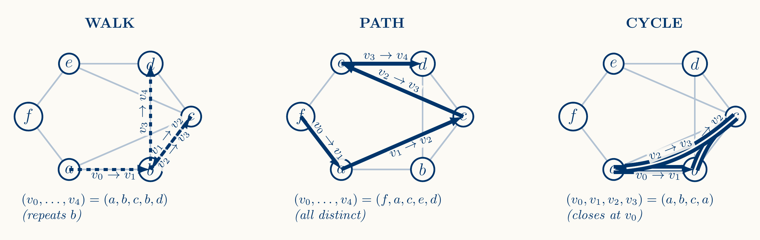
• A walk is a finite sequence of adjacent vertices:

  \[v_0...,v_t:\Set{v_{i-1},v_i} \in E \ \ \forall i \leq t \in \mathbb{N}\]

• A path is a walk with all the vertices distinct:

  \[v_0...,v_t:\Set{v_{i-1},v_i} \in E \land v_i \neq v_j \ \ \forall i,j \in \mathbb{N}\]

• A cycle is a walk $v_0,…,v_{t-1},v_0$ where $v_0,…,v_{t-1}$ is a path.

  

• A complete graph $G$ is a graph where every pair of vertices is connected by an edge:

  \[G := (V,E) : E = \binom{V}{2}\]

  Observe that this means that $\vert N(v)\vert = \vert V\vert - 1$.

Going back to isolated vertices, we say that

\[G \text{ is connected } \iff \forall u,v \in V \ \exists \text{ a path}: u,w_1...,w_{t-1},v\]

4.2.1.2. Graph coloring.

Being, $G := (V,E)$, then a $k\text{-coloring}$ of $G$ is an application:

\[c : V \to \Set{1,...,k} : \forall \Set{u,v} \in E \ \ c(u) \neq c(v)\]

For $G$, we define his chromatic number as the minimum number for which exists a coloration:

\[\chi(G) := min\Set{k | \exists c : V \to \Set{1,...,k} \text{ is a } k\text{-coloring}}\]

Observe that this means that the Four Colour theorem states $\chi(G) \leq 4 \ \ \forall G$ and the 3-coloring problem asks whether $\chi(G) \leq 3$.

Let's observe that:

1. For a complete graph $K_n$ (where $\vert V_K\vert = n$), is: $\chi(K_n) = n$.

   • First, let's see that $c : V_K \to \Set{1,…,n}$ is injective ($\vert V_K\vert = \vert \Set{1,…,n}\vert $) and it verifies:

     \[\forall u,v \in V_K : u \neq v \implies c(u) \neq c(v)\]

     Also, since $K_n$ is a complete graph, $\forall u,v \in V_K : u \neq v \iff \Set{u,v} \in E_K$, thus:

     \[\forall \Set{u,v} \in E_K \ \ c(u) \neq c(v)\]

     And $c$ is a coloration.

     
     

   • Let's see now that $\neg (\exists i < n : c : V_K \to \Set{1,…,i} \text{ is a coloration})$.

     Simply, considering $c : V_K \to \Set{1,…,i}$ with $ i < n$, then $c$ is not injective and it verifies the pigeonhole principle:

     \[\exists u,v \in V_K : u \neq v \land c(u) = c(v)\]

     Again, for $\forall u,v \in K_n \ \ u \neq v \iff \Set{u,v} \in E_K$ and thus:

     \[\exists \Set{u,v} \in E_K : c(u) = c(v)\]

     And $c$ is not a coloration.

     
     

2. For a cycle $C_n$, $\chi(C_n) = 2$ if $n$ is even and $\chi(C_n) = 3$ if $n$ is odd.

   First, let's define what a cycle graph is:

   \[C_n := (V_C, E_C) : \begin{cases} V_C = \Set{v_0,...,v_{n-1}} \\ E_C = \Set{\Set{v_{i-1},v_i} : i \in \Set{1,...,n-1}} \cup \Set{\Set{v_{n-1},v_0}} \end{cases}\]

   Let's observe that, as defined, the sequence: $v_0,…,v_{n-1}$ is a path, thus $v_0,…,v_{n-1},v_0$ is a cycle.

   • Now, consider the case $\exists m : n = 2m$, then, we define:

     \[c : V_C \to \Set{1,2} : c(v_i) = \begin{cases} 1 \ \text{ if } i \text{ is even}\\ 2 \ \text{ if } i \text{ is odd} \end{cases}\]

     It is clear that even and odd numbers alternates each in a consecutive numeric sequence. So:

     \[c(v_{i-1}) \neq c(v_i) \ \ \forall v_{i-1},v_i \in v_0,...,v_{n-1} \implies c(v_{i-1}) \neq c(v_i) \ \ \forall \Set{v_{i-1},v_i} \in E_C\]

     For the same reason, if $n$ is even, then $n-1$ is odd and $c(v_{n-1}) \neq c(v_0)$, thus, in conclusion:

     \[c(u) \neq c(v) \ \ \forall \Set{u,v} \in E_C\]

     And $c$ is a $2-coloring$ of $C_n$. Obviously since $E_C \neq \varnothing$ it can't be $\chi(C_n) = 1$.

     
     

   • If $n = 2m + 1$ and we suppose the existence of a $2-coloring$, $c$ over $C_n$, then:

     \(c(u) \neq c(v) \ \ \forall \Set{u,v} \in E_C \implies c(v_{i-1}) \neq c(v_i) \ \ \forall \Set{v_{i-1},v_i} \in E_C \iff\) \(\iff c(v_{i-1}) \neq c(v_i) \ \ \forall v_{i-1},v_i \in v_0,...,v_{n-1}\)

     Or, in other words, any consecutive vertex in the path $v_0,…,v_{n-1}$ has different image under $c$.

     Thus, is easy to see that:

     • Since in a $2-coloring$ there are only two possible images values

     • And $n-1$ is even (because $n$ is odd),

     Then $v_0$ and $v_{n-1}$ share the same image under $c$ and it is:

     \[c(v_{n-1}) = c(v_0) \land \Set{v_{n-1},v_0} \in E_C\]

     Triggering a contradiction with the $2-coloring$ requirement.

     Getting the example of $c$ provided above, is easy to see that:

     \[c : V_c \to \Set{1,2,3} : c(v_i) = \begin{cases} 1 \ \text{ if } i \text{ is even } \land i \neq n -1\\ 2 \ \text{ if } i \text{ is odd} \\ 3 \end{cases}\]

     Is a $3-coloring$ of $C_n$.

     
     

3. Bipartite Graphs.

   A bipartite graph is a graph $G_B$ satisfying:

   \[G_B := (V_B,E_B): \begin{cases}V_B := A \sqcup B \ \ (V = A\cup B \land A \cap B = \varnothing) \\ E_B \subset \binom{V_B}{2} : a \in A \land b \in B \ \ \forall \Set{a,b} \in E_B \end{cases}\]

   Then, consider

   \[c : V_B \to \Set{1,2} : c(v) =\begin{cases} 1 \ \ \text{ if } v \in A\\ 2 \ \ \text{ if } v \in B \end{cases}\]

   Then:

   \[\forall \Set{u,v} \in E_B \ \ \begin{cases} u \in A \Rightarrow c(u) = 1 \\ v \in B \Rightarrow c(v) = 2 \end{cases} \implies c(u) \neq c(v)\]

   And $c$ is a $2-coloring$ of $G_B$. Of course, $E_B \neq \varnothing \implies \chi(G_B) \neq 1$.

   
   

4. 2-colorability theorem.

   The 2-colorability characterization states that, being $G := (V,E)$ a graph, then:

   \[\chi(G)=2 \iff G \text{ is bipartite } \iff \neg \exists\,\text{cycle } C \subseteq G : |C|\ \text{ is odd}\]

   Observe that we already demonstrated that:

   • $G \text{ is bipartite } \implies \chi(G)=2$
   • $\chi(G)=2 \implies \neg \exists\,\text{cycle } C \subseteq G : \vert C\vert \ \text{ is odd}$ (since all odd cycle has a 3 as a chromatic number).

   • $\chi(G)=2 \implies G \text{ is bipartite }$

     Observe that

     \[\chi(G)=2 \implies \exists c :V \to \Set{1,2} : c(u) \neq c(v) \ \ \forall \set{u,v} \in E\]

     We define:

     \[\begin{cases}A := \Set{u \in V | c(u) = 1} \\ B:= \Set{u \in V | c(u) = 2}\end{cases}\]

     In this context, since $c$ is an application we have:

     • $v \in V \Rightarrow c(v) = 1 \vee c(v) =2 \Leftrightarrow v \in A \vee v \in B \Rightarrow V = A \cup B$

     • $A \cap B = \varnothing$

     • $\forall \Set{u,v} \in E \implies c(u) \neq c(v) \implies (u \in A \land v \in B) \vee (v \in A \land u \in B)$

     
     

     Thus, $G$ verifies: \(\begin{cases}V := A \sqcup B \ \ (V = A\cup B \land A \cap B = \varnothing) \\ E \subset \binom{V}{2} : a \in A \land b \in B \ \ \forall \Set{a,b} \in E \end{cases}\)

   Now, only last to demonstrate that:

   • $\neg \exists\,\text{cycle } C \subseteq G : \vert C\vert \ \text{ is odd} \implies G$ is bipartite.

     The premise can be negated in two ways:

     • First, $\neg \exists C \subseteq G : C \text{ is a cycle}$, then consider a vertex we call $r$ and: $A = \Set{u \vert dist(r,u) \text{ is even}}$ and $B = \Set{u \vert dist(r,u) \text{ is odd}}$. Then it is pretty obvious that $A \cup B$ and we impose that $A \cap B = \varnothing$; let's observe that this imposition requires no odd cycles.

       Being $C \subseteq G : C \text{ is odd}$, then, $C:=v_0,…,v_{n-1},v_0$ where $v_0,…,v_{n-1}$ is a path and $\Set{v_{n-1},v_0} \in E$. Let's say $r : dist(r,v_0) \land r \notin C$. Then, since $C$ is a cycle there are two paths to measure the distance between $r$ and $v_{n-1}$:

       \[dist(r,v_{n-1}) = dist(r,v_0) + dist(v_0,v_{n-1})\]

       Since $\Set{v_{n-1},v_0} \in E \Rightarrow dist(v_0,v_{n-1}) = 1 \Rightarrow dist(r,v_{n-1}) = 2 \text{ (even)}$, but also, since $C$ is odd, $n-1$ is even (meaning that $dist(v_0,v_{n-1})$ is even and $1 + dist(v_0,v_{n-1}) = dist(r,v_{n-1})$ is odd). So in summary: $A \cap B \neq \varnothing$

       
       

4.2.1.3. Planar graphs. Drawings and faces. Euler's formula.

A planar graph is a graph that admits a graphical representation on a plane such that its edges do not cross each other. For example, the complete graph $K_3$ does admit a representation in which the edges do not cross, but $K_5$ does not.

Let be $G:=(V,E)$ a finite simple graph, then an embedding of $G$ into $\mathbb{R}^2$ is a function $\phi: G \to \mathbb{R}^2$ that:

• $\forall u,v \in V \ \ \left(\phi(u), \phi(v) \in \mathbb{R}^2 \land u \neq v \implies \phi(u) \neq \phi(v) \right)$

• $\forall e, f \in E \ \ \left( \phi(e) = \gamma_{e_1e_2}, \phi(f) = \gamma_{f_1f_2} \in \mathbb{R}^2 : e \neq f \implies \phi(e) \cap \phi(f) \subseteq \Set{\phi(e_1),\phi(e_2),\phi(f_1),\phi(f_2)} \right)$

Where $\gamma_{uv}$ is a simple arc (non-self-intersecting, continuous curve) from $\phi(u)$ to $\phi(v)$. $\phi$ maps the edges of $G$ ensuring that two different arcs only share endpoints as much.

Then, $G$ is said to be planar if it admits an embedding $\phi$ in $\mathbb{R}^2$ as above.

Associated with a drawing of a planar graph are the so-called faces, grouped in the set $F$; which are regions of the plane $\mathbb{R}^2$ enclosed by the planar drawing of the graph (here the unbounded outer face external to the graph is included). Euler's formula specifies that, for a connected planar graph $G:= (V,E)$, being $F$ the set of the faces of the drawn graph, then:

\[|V| - |E| + |F| = 2\]

4.2.1.4. Dual graphs.

Given a connected planar graph $G$, the dual graph is what you get when you turn faces into vertices in a planar embedding of $G$.

The drawing (planar embedding) cuts the plane into regions (faces), one unbounded “outside” face plus the bounded ones, then the dual $G^*$ is built by:

• Putting one vertex inside each face of $G$.
• For each $e \in E$ there exists one $e^* \in E^*$ crossing once $e$, connecting two faces.

Formally;

Being $G$ a connected planar graph and $\phi$ his drawing in $\mathbb{R}^2$. Then, we define the dual graph as:

\[G^*:= (V^*,E^*):\begin{cases}V^* &:= F = \Set{f : f \text{ is a face of }(G,\phi)} \\ E^* &:= \Set{\Set{f_1,f_2} | \exists e \in E \text{ between } f_1 \text{ and } f_2 } \subseteq \binom{V^*}{2}\end{cases}\]

Is important to understand that Dual depends on the embedding: Two different planar drawings of the same abstract planar graph can produce non-isomorphic duals. The dual is canonical only after you fix the embedding.

In this context, a map coloring is equal to color a dual graph. A map representation is in fact a dual graph.

4.2.2. Formulating the problems. Three-coloring problem.

4.2.2.1. Describing the problem.

With the notions we have gathered, the Four Color Theorem (the “all maps” statement) states that, for every planar graph $G$, the chromatic number is at most 4, $\chi(G) \leq 4$. It only requires four colours to color every planar map.

However, for example $\chi(K_4)=4$, so three colors is not always sufficient. And we can formulate the problem as the language:

\[L := \Set{G | \chi(G)\leq 3}\]

However, in these terms, $G$ is still a graph and not a string codification of a graph, and it isn't a computable decision problem.

4.2.2.2. Graph Encoding.

Matrix reduction

Given a finite simple undirected graph $G :=(V,E) : \vert V\vert = d \in \mathbb{N}$, then consider the following elements:

• Being $[d] := \Set{1,…,d} \subset \mathbb{N}$ the function $T$ such:

  \[T: V \to [d] : \Big(u \neq v \Rightarrow T(u) \neq T(v) \Big)\ \ \ \forall v,u \in V\]

  Meaning that any vertex is mapped to a distinct natural number between $1$ and $\vert V\vert $. Observe that $T$ is bijective (our imposed condition makes it injective and since both domain and codomain have the same cardinal, from the injectivity we obtain the surjectivity and thus the bijectivity) and we can consider its inverse $T^{-1}$.

  
  

• The function $T'$ such:

  \[\begin{align}T'&: \binom{T(V)}{2} \to \Set{0,1} \\ T'(\Set{n,m}) &= \begin{cases} \ 1 \ \ \ \Set{T^{-1}(n),T^{-1}(m)} \in E \\ \ 0 \ \ \ \Set{T^{-1}(n),T^{-1}(m)} \notin E\end{cases}\end{align}\]

  We define $T'(E):=\Set{\Set{n,m} \vert T'(\Set{n,m}) = 1 } \subseteq \binom{T(V)}{2}$

  
  

• The matrix:

  \[M_{d} := (a_{ij})_{i,j \in T(V)} : a_{ij} = \begin{cases} \ 1 \ \ \ \Set{i,j} \in T'(E) \\ \ 0 \ \ \ \Set{i,j} \notin T'(E)\end{cases}\]

  This is called the edge matrix, and it stores the edges of $G$ in the form of entries equal to one. Since this is a symmetric matrix, we end up defining its upper part to avoid redundancies:

  \[M^+_{d} := (a^+_{ij})_{i,j \in T(V)} : a_{ij}^+ = \begin{cases} \ \ a_{ij} \ \ \ i < j \\ \ \ 0 \ \ \ \ \ \ i \geq j\end{cases}\]

In this context, we can reduce $G$ to $M^+_{d}$ in the sense that $M^+_d$ has all the necesary information to craft an equivalent graph $G_T$ of $G$:

\[M^+_d \to G_T \ := ([d], E_T) :E_T = \Set{\Set{i,j}:a^+_{ij} = 1 \land i < j}\]

Matrix Encoding

Let be:

\[M_n := (a_{ij})_{i,j \in [n]}\]

Then, we can reorganize the $a_{ij}$ elements by following rows:

\[\langle M_n \rangle : = (a_{11}...,a_{1n},a_{21},...,a_{nn}) = (\alpha_s)_{s \in [n^2]} : a_{ij} = \alpha_{n·(i-1) + j}\]

Let's see how to reconstruct $M_n$ from the sequence $(\alpha_s)_{s \in [n^2]}$.

Let's think that in $M_n$, each row is a group of $n$ elements and each column is a number between $1$ and $n$, thus the Euclidean division fits well, giving us as a final result:

\[(\alpha_s)_{s \in [n^2]} \to (a_{ij})_{i,j \in [n]}: \begin{cases} i =\left\lfloor \frac{s-1}{n}\right\rfloor +1 \\ j = ((s-1) \text{mod } n) +1 \end{cases}\]

Observe that each row of $M_n$ is a set of $n$ elements, thus it is in our interest to decompose any index $\alpha_m$ in terms of $n$ through the Euclidean Division theorem.

Being

\[\alpha_m \in (\alpha_s)_{s \in [n^2]} \implies \exists p,q \in \mathbb{N} : m = np + q \land 0 \leq q < n\]

Observe that this expression is telling us two things:

1. $p$ tells us how many times $n$ is contained in $m$. This is related to how many rows down $\alpha_m$ is as $a_{ij}$ on $M_n$.
2. $q$ is how much is left over for $m$ to be an $n$-multiple. This is related to how many columns to the left $\alpha_m$ has as $a_{ij}$ on $M_n$.

Both of them are related to the position of $\alpha_m$ as $a_{ij} \in M_n$ but not in a straightforward way.

Specifically, this equation has two problems:

• First, $q$ adjusts just fine to the column place $j$ in the sense that it correctly defines the position $p·n \leq m \leq (p + 1)·n$, but $q$ does not exist in an interval compatible with $j$, since $q \in [0,n-1] \cap \mathbb{N}$ and $j \in [n]$.

  Thus, we have to find a similar expression of the Euclidean division between $m$ and $n$ that fits $q$ in the correct set of values:

  \[m = np + q : 0 \leq q < n \iff m-1 = np+ (q-1) : 0 \leq q-1 < n \implies q\in [n]\]

  This expression correctly defines $q$ in a way compatible with $j$. Solving for $q$ we obtain:

  \[j = q = ((m-1)\text{mod } n) +1\]

  
  

• Now, we have a similar problem with the rows. As we said above, the expression tells us the number of times that $n$ fits in $m$. Translated to $M_n$, if $p=0 \implies i=1, p = 1 \implies i = 2$, and so on.

  Thus, $i = p + 1$, again solving we have:

  \[i = p + 1 = \left\lfloor \frac{m-1}{n}\right\rfloor +1\]

  Where $\left\lfloor \frac{a}{b}\right\rfloor$ denotes the integer division of $a$ by $b$.

  Note that, to obtain $i$, we did not solve from $m = p·n + q$ but from $m-1 = p·n + (q-1)$, since the latter accurately identifies $j \leftrightarrow q$; in the first expression this does not happen and thus there are inaccuracies in some edge cases like, for example, $m$ being a multiple of $n$.

4.2.2.3. Forming the problem.

Conceptual definition

Given a $G:=(V,E)$ and a function $c:V \to \Set{1,2,3}$, then if:

\[\forall \Set{u,v} \in E, \ c(u) \neq c(v) \iff c \text{ is a coloration on G} \implies \chi(G) \leq 3\]

This essentially means that, conceptually, we can ensure that $\chi(G) \leq 3$ if the function $c$ defined as above is indeed a coloration, by checking that there are no neighbouring vertices with the same color.

Formalizing the language

Given the alphabet $\Sigma = \Set{0,1}$, we just saw above that any graph can be reduced as follows:

\[G:=(V,E):\vert V \vert = n \ \simeq \ M^+_n := (a_{ij})_{i,j \in [n]} \ \simeq \ (\alpha_s)_{s\in[n^2]} \in \Sigma^*\]

Now, lets define:

\[c_T: [n] \to \Set{\alpha, \beta, \gamma} : c_T(i) = \begin{cases}\alpha \ \ \ \ c(u) = 1 \\ \beta \ \ \ \ c(u) = 2 \\ \gamma \ \ \ \ c(u) = 3 \end{cases} \ \ \land \ \ u = T^{-1}(i)\]

Observe that as defined; $c$ is a coloration on $G:=(V,E)$ iff $c_T$ is a coloration of $G_T:=([d],E_T)$, since:

\[c(u) \neq c(v) \ \ \forall \Set{u,v} \in E \iff c_T(i) \neq c_T(j) \ \ \forall \Set{i,j} \in E_T\]

Thus, applying $c_T$ to the sequence $(\alpha_s)_{s\in[n^2]}$ and the $i,j$ translation, the language to decide is:

\[L = \Set{(\alpha_s)_{s\in[n^2]} | \exists c_T : [n] \to \Set{\alpha, \beta, \gamma}: c_T\left(\left\lfloor \frac{s-1}{n}\right\rfloor +1\right) \neq c_T\left(((s-1) \text{mod } n) +1\right) \ \ \forall s : \alpha_s=1}\]

4.2.2.4. Verifying L.

In these terms, we can think of a verifier that admits a sequence and a function as described above, $V((\alpha_s)_{s\in[n^2]} ,c_T)$, and goes iterating over each term of the sequence $\alpha_s$ performing:

1. $\begin{cases} s \leq n(n-1) \to (1) \land \alpha_s (q_1) \\ s> n(n-1) \to \text{ACCEPT STATE}\end{cases}$

2. $\begin{cases} \alpha_s = 1 \to (2) \land \alpha_s \\ \alpha_s = 0 \to (0) \land \alpha_{s+1}\end{cases}$

3. $\begin{cases} c_T\left(\left\lfloor \frac{s-1}{n}\right\rfloor +1\right) = c_T\left(((s-1)\mod n) +1\right) \to \text{ REJECT STATE } \\ c_T\left(\left\lfloor \frac{s-1}{n}\right\rfloor +1\right) \neq c_T\left(((s-1)\mod n) +1\right) \to (0) \land \alpha_{s+1}\end{cases}$

Let's observe that, calling each step $p^s_i,q^s_i$ for the term $s$ of the sequence with $i=1,2,3$, a non-rejected path for the term $\alpha_s \in (\alpha_s)_{s\in[n^2]}$ by $V$ can be described as:

\[q^s_1 \vee (p^s_1 \land (q^s_2 \vee (p^s_2 \land q^s_3)))\]

Thus, for the $n(n-1)$ terms (observe that from the sequence we are eliminating those that correspond to the last row of $M_d^+$, which is zeroed) the complete accept path of $V((\alpha_s)_{s\in[n^2]},c_T)$ is:

\[\bigwedge_{s=0}^{n(n-1)} \left[q^s_1 \vee (p^s_1 \land (q^s_2 \vee (p^s_2 \land q^s_3)))\right]\]

Meaning that for each term, we check if it is $1$ or $0$ and if it is $1$, then we compare through $c_T$. By SAT, verifying an input of $L$ is equivalent to finding a valuation for that expression that makes it true.

5. Conclusion.

As a summary, in this section we saw what boolean formulas are and the NP SAT problem, which asks whether a boolean formula has a valuation making it true.

We also saw that SAT is NP-complete, meaning that it is hard enough (in complexity terms) to polynomially reduce any other NP problem to SAT, which eventually leads to the following corollary: any NP problem instance can be verified by verifying a SAT instance, this is; a correct valuation for a boolean formula that models the problem.

MathsFundamentals