<?xml version="1.0" encoding="utf-8"?><feed xmlns="http://www.w3.org/2005/Atom" ><generator uri="https://jekyllrb.com/" version="3.10.0">Jekyll</generator><link href="/feed.xml" rel="self" type="application/atom+xml" /><link href="/" rel="alternate" type="text/html" /><updated>2026-07-07T14:28:35+00:00</updated><id>/feed.xml</id><title type="html">GSanmi&apos;s blog</title><subtitle>Notes and papers on mathematics, cryptography, and theoretical computer science</subtitle><author><name>German Sanmi</name></author><entry xml:lang="en"><title type="html">Natural Numbers</title><link href="/posts/2026/06/17/NaturalNumbers/" rel="alternate" type="text/html" title="Natural Numbers" /><published>2026-06-17T09:00:00+00:00</published><updated>2026-06-17T09:00:00+00:00</updated><id>/posts/2026/06/17/NaturalNumbers</id><content type="html" xml:base="/posts/2026/06/17/NaturalNumbers/"><![CDATA[<h1 id="0-index">0. Index.</h1>

<h1 id="1-introduction">1. Introduction.</h1>

<p>We are going to present part of the basics of number theory, culminating in the demonstration of the fact that the root of any natural number is rational iff this natural number is a perfect square.</p>

<p>The results shown in the present post are a single deductive chain with no added ingredient that starts from a single premise axiom of the natural numbers $\mathbb{N}$ (good order) and stops at the irrationality of $\sqrt{2}$. The idea that is worth remembering throughout the paper is: the good order produces the division algorithm, the division algorithm produces Bézout, which is a result that translates divisibility into linearity, and that expands to the rest.</p>

<p><br /></p>

<h2 id="11-conventions">1.1. Conventions.</h2>

<p>Before starting, let's fix some conventions:</p>

<ul>
  <li>
    <p>Being $a,b \in \mathbb{Z}$ then we say "$b$ divides $a$" and write $b \mid a$ when:</p>

\[b \mid a \iff \exists k \in \mathbb{Z} : a = kb\]

    <p>Let's observe that divisibility respects linearity:</p>

\[c \mid a \wedge c \mid b \implies c \mid (ma + nb) \quad \forall m,n \in \mathbb{Z}\]

    <p><br /></p>
  </li>
  <li>
    <p>Being $a,b \in \mathbb{Z}: ab  \neq 0$, we call $gcd(a,b) = \max\Set{c \in \mathbb{N} : (c \mid a \wedge c \mid b)}$, this is the maximum integer that divides both numbers at once. Let's observe some interesting facts:</p>

    <ul>
      <li>$1 \in gcd(a,b) \quad \forall a,b \in \mathbb{Z}$</li>
      <li>
        <p>$\max \Set{|a|,|b|} \geq c \quad \forall c \in gcd(a,b)$, observe immediately that any greater number would not divide both of them so it is not in $gcd(a,b)$.</p>
      </li>
      <li>$gcd(a,b) = gcd(b,a) \quad \forall a,b \in \mathbb{Z}$</li>
      <li>
        <p>$gcd(a,b) &gt; 0 \quad \forall a,b \in \mathbb{Z}$</p>

        <p><br /></p>
      </li>
    </ul>
  </li>
</ul>

<h1 id="2-good-order-in-mathbbn-induction">2. Good Order in $\mathbb{N}$. Induction.</h1>

<h2 id="21-conceptual-presentation">2.1. Conceptual presentation.</h2>

<p>Having clarified these concepts, let's talk about the "good order" and the induction principle. This idea is expressed as a property of a set; a set is said to have good order or be well-ordered if it has a minimum, this is, a least element. In a more generic way; a good order is a total order in which any non-empty subset has a minimum.</p>

<p>The canonical example is the set of the natural numbers. This will be our departure point:</p>

<p><strong>$\mathbb{N}$ is a well-ordered set</strong></p>

<p><br /></p>

<p>Let's now talk about the induction principle which is tightly related to $\mathbb{N}$ and co-implies good order.</p>

<p><br /></p>

<h2 id="22-formal-definition-good-order">2.2. Formal definition. Good order.</h2>]]></content><author><name>German Sanmi</name></author><category term="Number Theory" /><category term="Maths" /><summary type="html"><![CDATA[0. Index.]]></summary></entry><entry xml:lang="en"><title type="html">Topology of Metric Spaces</title><link href="/posts/2026/06/17/BasicTopology/" rel="alternate" type="text/html" title="Topology of Metric Spaces" /><published>2026-06-17T09:00:00+00:00</published><updated>2026-06-17T09:00:00+00:00</updated><id>/posts/2026/06/17/BasicTopology</id><content type="html" xml:base="/posts/2026/06/17/BasicTopology/"><![CDATA[<h1 id="0-index">0. Index.</h1>

<ol>
  <li>
    <p>Introduction.</p>
  </li>
  <li>
    <p>Finite, Countable and Uncountable Sets.</p>

    <p><br /></p>
  </li>
</ol>

<h1 id="1-introduction">1. Introduction.</h1>

<p>First, let's explain why there is a topology chapter in an analysis book.</p>

<p>As we asserted in other chapter, Analysis is the study of the <em>limits</em>, and the limit is essentially a statement about closeness. Then, the <em>Topology</em> is the branch which isolates and study the notions of closeness, proximity or continuity in abstract without appealing to distances or metrics.</p>

<p>Hence, this topology chapter brings to the reader a precise vocabulary-kit in which the terms limit, continuity or convergence have complete sense. The hardest theorems of elementary analysis are, in fact, topological theorems.</p>

<p>Analysis emerges to give foundation to Calculus works which, before analysis, it worked with a non-fully-deployed but intuitive idea of limit, then called <em>infinitesimals</em>; $dx$. Primordial analysis stablished a first <em>limit</em> definition that, despite being rude, was mathematically accurate:</p>

\[\lim_{x \to a} f(x) = L \quad \Longleftrightarrow \quad \forall\,\varepsilon&gt;0\;\;\exists\,\delta&gt;0\;:\;0&lt;|x-a|&lt;\delta\implies |f(x)-L| &lt; \varepsilon\]

<p>Observe that this first definition involves the metric, this means that this limit idea is not property of the real field, is property of the space in which a proximity notion exists which is what the topology studies.</p>

<p>Later, topologic concepts rebuilt the limit concept in a simplier way, disregarding metrics and epsilons and using heavy geometric nuance.</p>

<p><br /></p>

<p>Thus, there is three level of abstractions. First let's barely introduce what the <em>open sets</em> are; an open set is a set in which all its points are interior points. Intuitively, this means that the set does not contain its boundary, allowing you to approach any element without stepping outside the set's limits.</p>

<p><br /></p>

<p>Thus:</p>

<ul>
  <li>
    <p>A <strong>topologic space</strong>; is a set $X$ along witha a collection of open subsets following three axioms.</p>
  </li>
  <li>
    <p>A <strong>metric space</strong>; is a particular case of toplogic space in which the open subsets gets generated with the metric. In some sense, an open set is a set in which every element has an "enviroment" of elements (defined by the metric) within the set, like a circule or sphere centered in the element which enterly falls inside the set.</p>
  </li>
  <li>
    <p>A <strong>euclidean space</strong> is a particular case of the metric space in which the metric is the <em>euclid norm</em>.</p>

    <p><br /></p>
  </li>
</ul>

<p>Thus, the topology introduced in this section is the <em>metric spaces topology</em>.</p>

<p><br /></p>

<h1 id="2-finite-countable-and-uncountable-sets">2. Finite, Countable and Uncountable Sets.</h1>

<p>We begin this section with a definition of the function concept.</p>

<p><br /></p>

<h2 id="21-functions-applications">2.1. Functions. Applications.</h2>

<h3 id="211-main-concepts">2.1.1. Main concepts.</h3>

<p>Consider two sets. $A,B \neq \varnothing$.</p>

<p>Then we define a <em>function</em> or application $f$ from $A$ to $B$ and we denote it as:</p>

\[f : A \to B\]

<p>This is a relation which connects each $x \in A$ to one $y \in B$. We denote $f(x)$ to the subset of elements of $B$ related with $x$ by $f$:</p>

\[f(x) := \Set{ y \in B \mid x \ \underbrace{\mapsto}_{f} \ y}\]

<p>Observe that we implicitly define a rule that every function $f$ must satisfy; $f(x)$ is a unary set, it only has one element and thus, through an economization of notation we simply state $f(x) = y$ when $f$ is a function:</p>

\[\forall x \in A \ \exists! y \in B : f(x) = y\]

<p>In this context we state that $A$ is the domain and $B$ is the codomain of $B$ which not necesarily coincide with the set of all the images of $A$ through $f$, denoted by $f(A) := \Set{y \in B \mid \exists x \in A : y = f(x)}$ and called <em>range</em> of $f$.</p>

<p><br /></p>

<h3 id="212-injectivity-surjectivity-and-bijectivity">2.1.2. Injectivity, Surjectivity and Bijectivity.</h3>

<p>Let's explore three important concepts about how relations connect input with outputs. Be $f : A \to B$ a application, then:</p>

<ul>
  <li>
    <p><strong>Inyective</strong>: We say that $f$ is <em>inyective</em> it verifies no colisions with images, formally:</p>

\[\forall x,y \in A : x \neq y \implies f(x) \neq f(y)\]

    <p><br /></p>
  </li>
  <li>
    <p><strong>Surjective</strong>: We say that $f$ is <em>surjective</em> when the range of $f$ coincide with the codomain $f(A) = B$, intuitively it has no gaps, every element on the codomain is reached:</p>

\[\forall y \in B \ \exists x \in A : f(x) = y\]

    <p><br /></p>
  </li>
  <li>
    <p><strong>Biyective</strong>: We say that $f$ is <em>biyective</em> when is a "one-to-one" correspondence between the elements of $A$ and $B$:</p>

\[\forall y \in B \ \exists ! x \in A : f(x) = y\]

    <p>Let's observe that $f$ is biyective if and only if is at the same time surjective and inyective.</p>
  </li>
</ul>

<p><br /></p>

<h3 id="213-inverse">2.1.3. Inverse.</h3>

<p>Consider $f : A \to B$ to been a relation. In this context we talk about a mappping of $A$ into $B$ through $f$, then we consider the inverse mapping from $B$ to $A$, denoted by $f^{-1}$ as:</p>

\[f^{-1} : B \to A \mid [ \ f^{-1}(y) = x \iff f(x) = y \ ]\]

<p>Let's observe that, if we now turn $f$ to be a function, $f^{-1}$ is a only a function if $f$ is biyective and obviously $f^{-1}$ is biyective as well. Note that:</p>

\[(f \circ f^{-1})(x) = f(f^{-1}(x)) = x = f^{-1}(f(x)) = (f^{-1} \circ f)(x)\]

<p>Thus, we assert that for any function $f$ the inverse function exists if and only if $f$ is biyective.</p>

<p><br /></p>

<h2 id="22-cardinality-count-finiteness">2.2. Cardinality. Count. Finiteness.</h2>

<p>The following section stablishes the mathematically notion of <em>count</em>. Let's present the tools used to count.</p>

<p><br /></p>

<p>First, let's introduce the <em>cardinality</em>. Take $A,B \neq \varnothing$, then we say that both sets has the same cardinality if we can define a biyection between them.</p>

<p>Let's observe that:</p>

<ul>
  <li>We can define a biyection over any set with himself (reflexivity).</li>
  <li>If a biyection is stablished from $A$ to $B$, then the inverse is a biyection of $B$ to $A$ (symmetric).</li>
  <li>
    <p>If there are biyection from $A$ to $B$ and from $B$ to $C$, the composition of the both is a biyection from $A$ to $C$ (transitivity).</p>

    <p><br /></p>
  </li>
</ul>

<p>Thus, we can define a <em>equivalent relation</em> around cardinality; two sets are equivalent if they share his cardinality.</p>

<p><br /></p>

<p>Now, let's introduce that in mathematics, count consist basically in measure the cardinality of a set, this is, to count is to relate the elements of a set with another set through a biyection. Let's explore this idea formally, let be $A$ some set:</p>

<ul>
  <li>
    <p>$A$ is <em>finite</em> if exists some $n \in \mathbb{Z}^+ : A \sim [n]$, remember that $[n] = \Set{1,2,\ldots,n}$. In this terms we say that $A$ has cardinality or <em>cardinal number</em> of $n$, $[n]$ is the canonical representant of the cardinal-equivalence class of $A$.</p>
  </li>
  <li>
    <p>$A$ is <em>infinite</em> if its not finite.</p>
  </li>
  <li>
    <p>$A$ is <em>countable</em> (or enumerable or denumerable) if $A \sim \mathbb{Z}^+$.</p>
  </li>
  <li>
    <p>$A$ is <em>at most countable</em> if its finite.</p>
  </li>
  <li>
    <p>$A$ is <em>uncountable</em> if $\nexists S \in \mathcal{P}(\mathbb{Z}^+)  : A \sim S$, note that this involves $\mathbb{Z}^+$ it self.</p>
  </li>
</ul>

<p>Note that with this notions two finite cardinal-equivalents sets $A, B$ has the same number of elements, but observe that with infinite sets the idea of have <em>the same number of elements</em> becomes quite vague but the biyection idea retains its clarity.</p>

<p><br /></p>

<p>Let's see an example with $\mathbb{Z}$ and $\mathbb{Z}^+$ and consider $f: \mathbb{Z}^+ \to \mathbb{Z}$:</p>

\[f(z) := \begin{cases} z/2 \quad z \in 2\mathbb{Z} \\ -\frac{z-1}{2} \quad z \notin 2\mathbb{Z} \end{cases}\]

<p>Observe that this function is injective and suprajective so is a biyection and $\mathbb{Z}$ and $\mathbb{Z}^+$ has the same cardinality.</p>

<p><br /></p>

<p>Observe that this happens despite the fact that $\mathbb{Z}^+ \subset \mathbb{Z}$, buy a finite set cannot be equivalent to one of its proper subsets.</p>

<p><br /></p>

<h2 id="23-sequences">2.3. Sequences.</h2>

<h3 id="231-definition">2.3.1. Definition.</h3>

<p>Let's introduce the notion of a <em>sequence</em>. Intuitively a sequence is an infinite sorted list. Formally, a sequence is a function $s : \mathbb{Z}^+ \to A : s(n) \in A$, where $A \neq \varnothing$.</p>

<p>This function contains two objects that characterizes the information and the set:</p>

<ul>
  <li>
    <p>An index over the elements of $A$, which is given by the preimage $n \in \mathbb{Z} : x = s(n) \to x_n$</p>
  </li>
  <li>
    <p>To each index, each position, there is only one element ocupping the slot (this is given by the fact that $s$ is a function) which is called the $n$-th term of the sequence. Observe that two terms of distinct index not need to be distinct.</p>
  </li>
</ul>

<p>We often call as $\Set{x_n}$ to the sequence.</p>

<p><br /></p>

<p>Observe some interesting relation between sequences and countable sets. Since every countable set is the range of a $1-1$ function defined on $\mathbb{Z}^+$, we may regard every countable set as the range of a sequence of distinct terms. Speaking more loosely, we may say that the elements of any countable set can be arranged in a sequence.</p>

<p><br /></p>

<h3 id="232-theorem-every-infinite-subset-of-a-countable-subset-is-countable">2.3.2. Theorem; Every infinite subset of a countable subset is countable.</h3>

<p>Take some $A \subset E$, such $E$ is countable and $A$ is not finite. Since $E$ is countable then exists some biyection $f : \mathbb{Z}^+ \to E$, then we can consider $g: \mathbb{Z}^+ \to A$ as follows; since $A \subset E$ then we can consider the range of $f$ over $A$. Then, each element of $f(A)$ has an index, and since $\mathbb{Z}^+ \subset \mathbb{N}$ has good order, then we can consider first some minimum index $m$ and then we can order $f(A)$ items through his index. Then, $g(1) = x_m$, and the sucesor of $x_m$ in $A$ receives $g(2)$ and so on, ultimately, we crafted a sequence, $g$ in $A$, thus $g$ is a biyection and $A$ is countable.</p>

<p><br /></p>

<h2 id="24-families-intersection-and-union-of-a-family-of-sets-countable-and-uncountable-example-sets">2.4. Families. Intersection and Union of a family of sets. Countable and Uncountable example sets.</h2>

<h3 id="241-definition">2.4.1. Definition.</h3>

<p>Let's now introduce the <em>family</em> languages, the indexes family sets and define the union and intersection of an arbitrary family set.</p>

<p><br /></p>

<p>Let $A$ and $\Omega$ be sets such each $\alpha \in A$ is asociated with a subset of $\Omega$, denoted by $E_\alpha \subset \Omega$. We denote as $\Set{E_\alpha}$ to set whose elements are the sets $E_\alpha$ and call it <em>collection</em> of sets or <em>family</em> of sets.</p>

<p><br /></p>

<h3 id="242-union-and-intersection-of-sets">2.4.2. Union and Intersection of sets.</h3>

<p>The union of the sets $E_\alpha$ is defined as:</p>

\[\bigcup_{\alpha \in A} E_\alpha := \Set{x \in \Omega \mid \exists \alpha \in A : x \in E_\alpha}\]

<p><br /></p>

<p>The intersection:</p>

\[\bigcap_{\alpha \in A} E_\alpha := \Set{x \in \Omega \mid x \in E_\alpha \quad \forall \alpha \in A}\]

<p><br /></p>

<h3 id="243-relation-between-unionintersection-and-sumproduct">2.4.3. Relation between Union/Intersection and Sum/Product.</h3>

<p>Many properties of unions and intersections are quite similar to those of sums and products; in fact, the words sum and product were sometimes used in this connection, and the symbols $\sum$ and $\prod$ were written in place of $\cup$ and $\cap$. The asociativity and distributivity laws comes from this very same laws in disjuntion and conjuntion.</p>

<p><br /></p>

<h3 id="244-cantors-diagonal-methods-and-auxiliary-results">2.4.4. Cantor's diagonal methods and auxiliary results.</h3>

<p>We have the following results:</p>

<p><strong>The arbitrary union of countable sets is a countable set. First Cantor's diagonal method.</strong></p>

<p>Let' be $\Set{E_n} : n = 1,2,3,\ldots$ be a collection or family of countable sets, then consider:</p>

\[S = \bigcup_{i=1}^\infty E_n\]

<p>First, since $E_n$ for each $n =1,2,3,\ldots$ is numerable, then we can consider a biyection $f : \mathbb{Z}^+ \to E_n$ for each $n$, this biyection allow us to arrange or list the elements of $E_n$ in a row</p>

\[E_n :=\Set{x_{1n}, x_{2n}, x_{3n}, \ldots}\]

<p>Let's do this for each $n$ obtaining something like a matrix where each row is the sorted $E_n : n = 1,2,3,\ldots$</p>

\[S =\begin{pmatrix} x_{11} &amp; x_{12} &amp; x_{13} &amp; \ldots \\ x_{21} &amp; x_{22} &amp; x_{23} &amp; \ldots \\ x_{31} &amp; x_{32} &amp; x_{33} &amp; \ldots \\ \vdots &amp; \vdots &amp; \vdots &amp; \ddots \end{pmatrix}\]

<p>Note that the 'matrix' denomination of this structure is just an intuitive approximation and we are not saying that it is properly a matrix at all.</p>

<p>Then, observe we can sort this elements by diagonalizating them, forming the sequence:</p>

\[x_{11}, x_{21},  x_{12},  x_{31},  x_{22},  x_{13}, \ldots\]

<p>Observe then that as an arranged list, we can define a biyection over it, thus $S$ is countable.</p>

<p><br /></p>

<p><strong>The at most countable union of at most countable sets is at most countable</strong></p>

<p>The proof is similar to the above.</p>

<p><br /></p>

<p><strong>If $A$ is countable, then $A^n$ is countable for any $n \in \mathbb{N}$</strong></p>

<p>Let's proof this result by induction.</p>

<p>Take $n = 1$, then this result is immediate since $A^1$ is $A$.</p>

<p>Then, let's give it true for some $n \in \mathbb{N}$, and consider $A^{n}$, each element is of the form $(a_1,\ldots, a_{n-1}, a_n) \in A^n$, calling $\alpha = (a_1,\ldots,a_{n-1}) \in A^{n-1}$, then the first is identifiable with the pair $(\alpha,a_n)$, observe that fixed some $\alpha$, the set of the pairs $(\alpha,a) : a \in A$ can be identified with $A$ it self, meaning that is countable and his elements can be arranged in a row:</p>

\[(\alpha,a_1)_1,(\alpha,a_2)_2,(\alpha,a_3)_3,\ldots\]

<p>Also observe that since $A^{n-1}$ is countable as well, then, for each $a \in A$ the set of the pairs $(\alpha,a) : \alpha \in A^{n-1}$ is countable as well and it can be disposed in a column, obtaining a structure in which we can use the first Cantor diagonal method.</p>

\[(\alpha_1,a_1),(\alpha_1,a_2),(\alpha_1,a_3),\ldots\]

\[(\alpha_2,a_1),(\alpha_2,a_2),(\alpha_2,a_3),\ldots\]

\[(\alpha_3,a_1),(\alpha_3,a_2),(\alpha_3,a_3),\ldots\]

\[\quad \quad \vdots \quad \quad \quad \quad \vdots \quad \quad \quad \quad \vdots \quad \quad \quad\]

<p>Allowing us to create the sequence:</p>

\[(\alpha_1,a_1)_1,(\alpha_2,a_1)_2, (\alpha_1,a_2)_3, (\alpha_3,a_1)_4, (\alpha_2,a_2)_5, (\alpha_1,a_3)_6,\ldots\]

<p>Reidentificating the pair $(\alpha,a)$ with the tuple $(a_1,\ldots,a_n) \in A^n$, we have created a biyection from $\mathbb{Z}^+$ over the elements of $A^n$, so this is is countable as well.</p>

<p><br /></p>

<p>Essentially observe that we reused the argument provided in the first point since $A^n$ is the countable union of the countable sets $\Set{(\alpha,a) : a \in A}$ for each $\alpha \in A^{n-1}$, so is countable.</p>

<p><br /></p>

<p><strong>$\mathbb{Q}$ is countable</strong></p>

<p>Observe that we can again reuse the argument before. We did see that $\mathbb{Z}$ is countable so each set $E_m = \Set{n/m : n \in \mathbb{Z}}$ for some $m \neq 0$ is countable, thus:</p>

\[\mathbb{Q} := \bigcup_{m \in \mathbb{Z}^+}E_m\]

<p>Is countable.</p>

<p><br /></p>

<p><strong>Uncountable set. Second Cantor's diagonal method. $\mathbb{R}$ is uncountable.</strong></p>

<p>This is an example of an infinity which is strictly greater than $\mathbb{N}$. Consider the set $A:=\Set{0,1}^\mathbb{N}$, of all the functions $s:\mathbb{N} \to \Set{0,1}$. Observe that each sequence is the <em>indicator</em> function of some subset of $\mathbb{N}$, for which is in biyection with $\mathcal{P}(\mathbb{N})$, hence the theorem is $card(\mathbb{N}) \leq card(\mathcal{P}(\mathbb{N}))$.</p>

<p><br /></p>

<p>Take $E \subseteq A$ as countable consisting in the sequences $s_1,s_2,s_3,\ldots$. Then, take some sequence $s$ crafted as:</p>

<p>If the $n$-th digit in $s_n$ is $1$, then the $n$-th digit of $s$ is $0$ provoking that $s$ differs from any element of $E$ in at least one place so $s \notin E$ but $s \in A$ since $s$ is composed of $0$ and $1$ so $E \subset A$. Any countable subset of $A$ is a proper subset, thus $A$ can't be countable (or it would be its own countable subset) and is uncountable.</p>

<p><br /></p>

<p>Laterly we will see that $\mathbb{R}$ admits a binary representation and this same result will apply to demonstrate that $\mathbb{R}$ is uncountable.</p>

<p><br /></p>

<h2 id="25-summary">2.5. Summary.</h2>

<p>Let's take a brief summary of section $2$. First, we introduce the relation and a concrete form or relation which we called <em>function</em>, which is a relation for which the image set for any element of the domain is a unary-non-empty set.</p>

<p>Then we introduced the biyection, or one-to-one relations and along with it the mathematically conception of <em>count</em> which is identify the elements of two sets through a biyection in the sense that we can attach each element with another unique item of other set, stablishing that both sets has the same number of elements, the same cardinality. The cardinality equivalence is a relation equivalence in which the canonical representant is the natural number subsets, $[n]$.</p>

<p>Later</p>

<h1 id="3-metric-spaces">3. Metric Spaces.</h1>

<p><br /></p>]]></content><author><name>German Sanmi</name></author><category term="Analisis Rudin" /><category term="Maths" /><summary type="html"><![CDATA[0. Index.]]></summary></entry><entry xml:lang="en"><title type="html">Euclidean Space</title><link href="/posts/2026/06/16/EuclideanSpaces/" rel="alternate" type="text/html" title="Euclidean Space" /><published>2026-06-16T09:00:00+00:00</published><updated>2026-06-16T09:00:00+00:00</updated><id>/posts/2026/06/16/EuclideanSpaces</id><content type="html" xml:base="/posts/2026/06/16/EuclideanSpaces/"><![CDATA[<h1 id="0-index">0. Index</h1>

<ol>
  <li>Presentation and Definition. $\mathbb{R}^k$</li>
  <li>Metric Spaces.
    <ul>
      <li>2.1. Metric definition. Metric spaces.</li>
      <li>2.2. Euclidean metric.</li>
      <li>2.3. $\mathbb{R}^k$ is a metric space with the euclidean metric.</li>
    </ul>
  </li>
  <li>Main properties of the norm in $\mathbb{R}^k$.</li>
  <li>
    <p>Summary.</p>

    <p><br /></p>
  </li>
</ol>

<h1 id="1-presentation-and-definition-mathbbrk">1. Presentation and Definition. $\mathbb{R}^k$</h1>

<p>A <em>Euclidean space</em> is an affine space over the reals such that the associated vector space is a euclidean vector space; a finite-dimensional inner product space over the real numbers.</p>

<p>Let's consider the affine space $(\mathbb{R}^k,V,+)$ where the associated $\mathbb{R}$-vector space is $V= (\mathbb{R},(\mathbb{R}^k,+),·)$, with the operations as follows:</p>

\[(x_1,...,x_k)+(y_1,...,y_k)=(x_1+y_1,...,x_k+y_k)\]

\[\alpha · (x_1,...,x_k) = (\alpha x_1,..., \alpha x_k)\]

<p>Being $+: V \times \mathbb{R}^k \to \mathbb{R}^k $ a simply transitive action over $\mathbb{R}^k$</p>

<p><br /></p>

<p>Over $V$, we define the following inner product, which we remember from the <a href="https://gsanmi1.github.io/posts/2026/03/05/Complex_Numbers/">Complex Numbers</a> post, on $6.3.1$.</p>

<p>An inner product is the object which injects geometry by defining how a vector expresses its own direction (norm), introducing subsequently the orthogonality. In this particular presentation, this inner product receives the particular name <em>dot product</em>.</p>

\[\quad \quad \langle x,y \rangle = x · y =\sum_{i=1}^k x_iy_i\]

<p><br /></p>

<p>The defined <em>dot product</em> gives rise to the <em>norm</em>; for each vector $x \in \mathbb{R}^k$ it is defined:</p>

\[\|x\| = \sqrt{ x·x}= \sqrt{\sum_{i=1}^k x_i^2}\]

<p>Which gives us a notion of "length" of the vector. It is worth saying that this is specifically true in $\mathbb{R}^k$ where intuitive geometry matches the formal geometry instituted through the dot product.</p>

<p><br /></p>

<p>Thus, a euclidean space is the result of injecting geometry into an affine space through a real inner product space; a real vector space with geometry.</p>

<p>As a consequence of the geometry injected by the inner product, we can consider a notion of proximity (metric) between the points in the affine space which allows us to introduce the notion of limit and develop the analysis.</p>

<p><br /></p>

<h1 id="2-metric-spaces">2. Metric spaces.</h1>

<h2 id="21-metric-definition-metric-spaces">2.1. Metric definition. Metric spaces.</h2>

<p>A metric abstracts the notion of <em>distance</em>. This is an important concept since from this all the analysis departs. From the distance notion comes proximity and then limits gain sense.</p>

<p>A <em>distance</em> tries to capture how far two points are from each other in a non-empty set $X$. Observe that this is not an algebraic structure or algebraic property; contrary to the norm, the distance doesn't need to sum or scale.</p>

<p><br /></p>

<p>Let $X$ be a non-empty space, then a <em>metric space</em> is a pair $(X,d)$ where: $d : X \times X \to \mathbb{R}$ is an application called <em>distance</em>, verifying:</p>

<ul>
  <li>
    <p>$M1$: Symmetry, the distance is indifferent to the point of measurement:</p>

\[d(x,y)=d(y,x) \quad \forall x,y \in X\]

    <p><br /></p>
  </li>
  <li>
    <p>$M2$: Gets null on the diagonal:</p>

\[d(x,y)=0 \iff x = y \quad \forall x,y \in X\]

    <p><br /></p>
  </li>
  <li>
    <p>$M3$: Triangular inequality:</p>

\[d(x,z) \leq d(x,y) + d(y,z) \quad \forall x,y,z \in X\]

    <p><br /></p>
  </li>
</ul>

<p>Observe some immediate consequences of the three axioms:</p>

\[d(x,x) = 0 \leq d(x,y) + d(y,x) = 2d(x,y) \implies 0 \leq d(x,y) \quad \forall x,y \in X\]

<p><br /></p>

<p>The distance is always positive as a consequence of the triangular inequality and the symmetry.</p>

<p><br /></p>

<h2 id="22-euclidean-metric">2.2. Euclidean metric.</h2>

<p>Let's consider again the affine space $\mathbb{R}^k$ as defined above with the dot product. Then, $V$ is an inner product vector space and, consequently, a normed vector space. Let's see how we can develop a metric in $\mathbb{R}^k$ to state it as a metric space.</p>

<p>First, at this point, we will develop the metric in $\mathbb{R}^k$ through its norm (depending on the inner product) although we established this is not entirely necessary.</p>

<p><br /></p>

<p>We define the metric in $\mathbb{R}^k$ as, for $x,y \in \mathbb{R}^k$, we have that:</p>

\[d(x,y) = \|\overrightarrow{xy}\| = \|y - x\|\]

<p>This is, the distance between two points on $\mathbb{R}^k$ is the length of the vector that connects both points. Remember from our knowledge of affine space that $x + \overrightarrow{xy} = y$</p>

<p><br /></p>

<h2 id="23-mathbbrk-is-a-metric-space-with-the-euclidean-metric">2.3. $\mathbb{R}^k$ is a metric space with the euclidean metric.</h2>

<p>Let's see that $(\mathbb{R}^k,d)$ as defined is a metric space:</p>

<ul>
  <li>
    <p><strong>Symmetry</strong>:</p>

\[d(x,y) = \|x - y\| = \sqrt{\sum_i^k (x_i -y_i)^2} = \sqrt{\sum_i^k (y_i - x_i)^2} = \| y - x \|  = d(y,x)\]

    <p><br /></p>
  </li>
  <li>
    <p><strong>Zero distance along the same point:</strong></p>

\[d(x,y) = \|x - y\| = \sqrt{\sum_i^k (x_i -y_i)^2}\]

    <p>Since it is a sum of positive terms, to be zero all the operands have to be zero, this is:</p>

\[d(x,y) = 0 \iff x_i =y_i \quad i=1,2,...,k \iff x = y \quad \forall x,y \in \mathbb{R}^k\]

    <p><br /></p>
  </li>
  <li>
    <p><strong>Triangle inequality</strong>: This result comes immediately from the inner product. Take $x,y \in \mathbb{R}^k$, then:</p>

\[\|x+y\|^2 = \|x\|^2 + \|y\|^2 + 2 \langle x,y \rangle\]

    <p>Let's see that, by Cauchy-Schwarz: $|\langle x,y \rangle| \leq ||x|| ||y||$, thus</p>

\[\|x+y\|^2 = \|x\|^2 + \|y\|^2 + 2 \langle x,y \rangle \leq \|x\|^2 + \|y\|^2 + 2\|x\| \|y\| = (\|x\| + \|y\|)^2\]

    <p>Since $||x+y|| \geq 0$ and $||x|| + ||y|| \geq 0$ is:</p>

\[\|x+y\|^2 \leq (\|x\| + \|y\|)^2 \implies \|x+y\| \leq \|x\| + \|y\|\]

    <p>Giving place to the triangular inequality (which is always true in a real inner product space).</p>

    <p><br /></p>

    <p>Now, observe that:</p>

\[d(x,z) = \|x -z\| = \|x -y + y-z\| \leq \|x-y\| + \|y-z\| = d(x,y)+d(y,z)\]

    <p>The inequality is guaranteed by the triangle inequality in the norm, preceded by Cauchy-Schwarz.</p>

    <p><br /></p>
  </li>
</ul>

<h1 id="3-main-properties-of-the-norm-in-mathbbrk">3. Main properties of the norm in $\mathbb{R}^k$</h1>

<p>Let's evaluate some main properties of the norm of $\mathbb{R}^k$.</p>

<ol>
  <li>$||x|| \geq 0$, is immediate from the fact that is the square of a real number.</li>
  <li>$||x|| = 0 \iff x = 0$, immediate from norm definition.</li>
  <li>$||\alpha x || = (\langle \alpha x, \alpha x \rangle)^\frac{1}{2} = (\alpha^2 \langle x,x \rangle)^\frac{1}{2} = |\alpha| ||x||$</li>
  <li>$||x · y|| \leq ||x|| ||y||$ Immediate from Cauchy-Schwarz.</li>
  <li>$||x+y|| \leq ||x|| + ||y||$ Triangle inequality previously demonstrated.</li>
  <li>
    <p>$||x-z|| \leq ||x-y|| + ||y-z||$ An extension of the triangle inequality relative to the euclidean metric also demonstrated above.</p>

    <p><br /></p>
  </li>
</ol>

<h1 id="4-summary">4. Summary.</h1>

<p>Thus, we've seen that $\mathbb{R}^k$ as an affine space with $\mathbb{R}^k$ as the associated vector space and the real inner product as the dot product; $x · y$ conforms a Euclidean space; an affine space with a geometry induced by the vector space which crystallizes in the metric $d(x,y) = ||\overrightarrow{xy}||$</p>

<p><br /></p>

<h1 id="5-exercises">5. Exercises.</h1>

<h2 id="51">5.1.</h2>

<table>
  <tbody>
    <tr>
      <td>Suppose $k \geq 3$, $x,y \in \mathbb{R}^k :</td>
      <td>x-y</td>
      <td>= d &gt; 0$ and $r&gt;0$. Prove:</td>
    </tr>
  </tbody>
</table>

<ol>
  <li>
    <p>If $2r &gt; d$ there are infinitely many $z \in \mathbb{R}^k$ such:</p>

\[|z - x| = |z - y| = r\]

    <p>Observe that by the triangle inequation is:</p>

\[|x -y| \leq |x-z| + |z-y|\]

    <p>Thus, the points requested by the exercise are those points satisfying:</p>

\[z \in \mathbb{R}^k: \begin{cases}|x-z| = |z-y|\\ d = |x -y| &lt; |x-z| + |z-y| = 2r\end{cases}\]

    <p>Note that the first condition give us a general caracterization of the points $z$, those whose coordinates satisfies the equation:</p>

\[\left(\sum_{i=1}^k(x_i - z_i)^2\right)^{1/2} = \left(\sum_{i=1}^k(y_i - z_i)^2\right)^{1/2}  \iff \sum_{i=1}^k(x_i - z_i)^2 = \sum_{i=1}^k(y_i - z_i)^2\]

    <p>Note that for each square is:</p>

\[(x_i - z_i)^2 = x^2_i -2x_iz_i + z^2_i = y^2_i -2y_iz_i + z^2_i = (y_i - z_i)^2\]

    <p>The $z^2_i$ cancels from both sides and sorting:</p>

\[2z_i(y_i - x_i)=y^2_i - x^2_i\]

    <p>Adding now the summatories we have:</p>

\[z·(y-x) = \frac{1}{2}(|y|^2 - |x|^2)\]
  </li>
</ol>]]></content><author><name>German Sanmi</name></author><category term="Maths" /><category term="analisis_rudin" /><category term="Maths" /><summary type="html"><![CDATA[0. Index]]></summary></entry><entry xml:lang="en"><title type="html">3. VectorSpaces Properties</title><link href="/posts/2026/06/08/VectorSpacesProperties/" rel="alternate" type="text/html" title="3. VectorSpaces Properties" /><published>2026-06-08T09:00:00+00:00</published><updated>2026-06-08T09:00:00+00:00</updated><id>/posts/2026/06/08/VectorSpacesProperties</id><content type="html" xml:base="/posts/2026/06/08/VectorSpacesProperties/"><![CDATA[<h1 id="0-index">0. Index.</h1>

<ol>
  <li>Introduction.</li>
  <li>Subspaces.
    <ul>
      <li>2.1. Definition and characterization.</li>
      <li>2.2. Example of subspaces.</li>
      <li>2.3. Combination of vector spaces.
        <ul>
          <li>2.3.1. Intersection of subspaces.</li>
          <li>2.3.2. Spanned subspace by a set.</li>
          <li>2.3.3. Sum of subsets of vector spaces.</li>
        </ul>
      </li>
      <li>2.4 Example of combinated vector spaces.
        <ul>
          <li>2.4.1. Subspace defined by equations.</li>
          <li>2.4.2. Matrix.</li>
          <li>2.4.3. Row-spaces.</li>
          <li>2.4.4. Caracterization of the polynomial vectorspace.</li>
          <li>
            <p>2.4.5. Subspaces exercises.</p>

            <p><br /></p>
          </li>
        </ul>
      </li>
    </ul>
  </li>
</ol>

<h1 id="1-introduction">1. Introduction.</h1>

<p>In the past post; <a href="https://gsanmi1.github.io/posts/2026/04/08/VectorSpaces/">Vector Spaces</a>, we've introduced that a vector space $(K,V,·)$ is the algebraic structure resulting from using a field $K$ to weigh the compositions of an abelian group $V$, through a field action $·$. Meaning that a vector space is a triple $(K,V, ·)$ where:</p>

<ul>
  <li>$K$ is a field.</li>
  <li>$V$ is an abelian (commutative) group.</li>
  <li>$· : K \times V \to V$ is a field action, which acts over $V$ using $K$'s elements to scale vectors, making families of <em>proportional vectors</em>.</li>
</ul>

<p>The resulting compositions are what we call <em>linear combinations</em>, independent contributions of the group's elements mediated by the field's scalars:</p>

\[\alpha v + \beta u : \alpha ,\beta \in \mathbb{R}, v,u \in V\]

<p>We presented some examples of sets which, with proper operations involved, are examples of vector spaces:</p>

<ul>
  <li>The $n$-tuples space: $F^n$</li>
  <li>The space of $m \times n$ matrices: $M_{m \times n}(F)$</li>
  <li>The space of functions from a set $S$ to a field $K$: $K^S$</li>
  <li>
    <p>The space of polynomial functions over a field K</p>

    <p><br /></p>
  </li>
</ul>

<p>We also developed, surreptitiously, the affine space structure, which is the way in which we use vectors to study a non-empty set in a simply transitive way, and we defined the <em>arrow</em> concept as the segment that connects two points of the affine space with magnitude, direction and orientation, which captures the displacement from the point at the base of the segment to the one lying at the end of the arrow.</p>

<p>We also demonstrated that if you fix one point $O$ and consider the family of all possible arrows with base at $O$, then that family has the structure of a vector space, which leaves us with a geometric intuition of what a vector is.</p>

<p><br /></p>

<p>Then, with this information as a starting point, let's develop the fundamental properties of vector spaces.</p>

<p><br /></p>

<h1 id="2-subspaces">2. Subspaces.</h1>

<h2 id="21-definition-and-characterization">2.1. Definition and characterization.</h2>

<p>In this section we shall introduce some of the basic concepts in the
study of vector spaces.</p>

<p><strong>Let $V$ be a vector space over the field $F$. A subspace of $V$ is a non-empty subset $W$ of $V$ which is itself a vector space over $F$ with the operations of vector addition and scalar multiplication on $V$.</strong></p>

<p><br /></p>

<p>Let's observe that, from the axioms of vector spaces, if $W$ is a vector space such $W \subset V$, then:</p>

<ul>
  <li>
    <p>Closure relative to linear combinations:</p>

\[v,u \in W \implies (\alpha v + \beta u \in V \ \forall \alpha, \beta \in  F)\]
  </li>
  <li>
    <p>Contains zero vector: $0_V \in W$, or $0_W = 0_V$. Remember that $V$ being a vector space means that $(V,+)$ is an abelian group, so $(W,+)$ is an abelian subgroup of $V$ and it inherits $0_V$ from $V$ by the uniqueness of this element. (Observe that this also extends to associativity and inverses).</p>

    <p><br /></p>
  </li>
</ul>

<p>Let's take a characterization for any non-empty subset $W \subset V$ to be a vector space. If $V$ is a $K$-vector space, then:</p>

\[W \text{ is a vector space } \iff (\alpha u + v \in W \quad \forall u,v \in W, \alpha \in K)\]

<p>Let's reconstruct the structure:</p>

<ul>
  <li>
    <p>$(W,+)$ is an abelian subgroup of $(V,+)$.</p>

    <p>Since $W \neq \varnothing$ (by the premise), we can consider $u,v \in W$, then: $(-1)u + v = v - u \in W$, so it is a subgroup of $V$. Let's see that $W$ also inherits commutativity from $V$ so it is an abelian subgroup.</p>

    <p><br /></p>
  </li>
  <li>
    <p>$· |_W: K \times W \to W$ is a field action:</p>

    <ul>
      <li>
        <p>Observe that $-1 u + u = 0 \in W$, thus $1 u + 0 = u \in W$ so the unit in $F$ doesn't change the vector and it falls inside $W$.</p>
      </li>
      <li>
        <p>Take some $v \in W \implies \alpha v + 0 = \alpha v \in W \implies \beta (\alpha v) + 0 = \beta (\alpha v) \in W$. For the same reason $(\alpha \beta)v \in W$. Then observe that in $V$, by associativity, is $\beta (\alpha v) = (\beta \alpha)v$ so both elements are equal in $V$ and the same in $W$ (by unicity of the inverse), thus $\beta (\alpha v) = (\beta \alpha)v$</p>
      </li>
      <li>
        <p>Take $(\alpha + \beta)v + 0 = (\alpha + \beta)v \in W \subset V$, then in $V$ is $(\alpha + \beta)v = \alpha v + \beta v$ so, for the same argument as above, is $(\alpha + \beta)v = \alpha v + \beta v$ in $W$.</p>
      </li>
      <li>
        <p>Take $\alpha v + 0 \in W \implies \exists w = \alpha v \in W$, take now other $u \in W$, then  $\alpha u + w \in W$, again in $V$ is $\alpha u + w = \alpha u + \alpha v = \alpha(u + v)$ and again is $ \alpha(u + v) = \alpha u + \alpha v$ in $W$.</p>
      </li>
    </ul>

    <p><br /></p>
  </li>
</ul>

<h2 id="22-example-of-subspaces">2.2. Example of subspaces.</h2>

<p>Let's consider some well-known examples of subspaces. Consider some $V$ a $K$-vector space, then:</p>

<ol>
  <li>$V$ is a subspace of $V$.</li>
  <li>
    <p>$\Set{0} \subset V$ is the <strong>zero subspace</strong> of $V$; $\alpha 0 + 0 = 0 \in \Set{0} \quad \forall \alpha \in K$ so $\Set{0}$ is a subspace of $V$.</p>
  </li>
  <li>
    <p>$A:= \Set{x \in K^n \mid x_1 = 0}$ is a subspace of $K^n$, check that always $\alpha x + y \in A$, trivially.</p>

    <p>But let's observe that $B := \Set{x \in K^n \mid x_1 = 1 + x_2}$ (the solution of a non-homogeneous equation) does not satisfy the rule, take some $\alpha$ and observe that:</p>

\[\alpha x + y = (\alpha (1 + x_2) + 1 + y_2), \alpha x_2 + y_2,..., \alpha x_n + y_n)\]

    <p>Then, $\alpha + 1 + \alpha x_2 + y_2 = 1 + \alpha x_2 + y_2 \iff \alpha=0$.</p>

    <p>So we have that $\forall \alpha \neq 0 \quad (x,y \in B \implies \alpha x + y \notin B)$</p>

    <p><br /></p>
  </li>
  <li>
    <p>The <strong>space of polynomial functions</strong> over $K$;</p>

\[\operatorname{Pol}(K, K) := \left\{\, f \in K^K \ \middle|\ \exists n \in \mathbb{N}_0,\ \exists (\alpha_0, \ldots, \alpha_n) \in K^{n+1} : \forall s \in K,\ f(s) = \sum_{i=0}^{n} \alpha_i\, s^i \,\right\}\]

    <p>Is a subspace of $K^K$.</p>

    <p>Observe that, if we get $f,g \in Pol(K,K)$, then is: $ f(s) = \sum_{i=0}^{n} \alpha_i\, s^i$, $g(s) = \sum_{i=0}^{m} \beta_i\, s^i$, consider is $n \leq m$, then we can expand $f(s)$ to $\sum_{i=0}^{m} \alpha_i\, s^i = \sum_{i=0}^{n} \alpha_i\, s^i +\sum_{i=n+1}^{m} 0\, s^i$ and then is:</p>

\[(\gamma f + g)(s) = \gamma f(s) + g(s) = \gamma \sum_{i=0}^{m} \alpha_i\, s^i  + \sum_{i=0}^{m} \beta_i\, s^i =\]

\[\sum_{i=0}^{m} \gamma\alpha_i\, s^i + \sum_{i=0}^{m} \beta_i\, s^i = \sum_{i=0}^{m} (\gamma\alpha_i + \beta_i) s^i = \sum_{i=0}^m \varphi_i \, s^i \in Pol(K,K)\]

    <p><br /></p>
  </li>
  <li>
    <p>Consider $S:=\Set{(a_{ij})<em>{ij} \in M_n(K) \mid (a</em>{ij})<em>{ij} = (a</em>{ij})_{ji}}$, the <strong>set of all symmetric matrices</strong> form a subspace of $M_n(K)$</p>

    <p>Take, $A,B \in S$, then let's see that $\alpha A + B = \alpha (a_{ij})<em>{ij} + (b</em>{ij})<em>{ij} = (\alpha a</em>{ij} + b_{ij})_{ij}$, then let's see that this matrix is in $S$ by observing that:</p>

\[A \in S \implies a_{ij} = a_{ji} \quad \forall i,j \implies \alpha a_{ij} = \alpha a_{ji} \quad \forall i,j  \implies \alpha A \in S\]

    <p>Now, observe that:</p>

\[A,B \in S \implies \begin{cases}a_{ij} = a_{ji} \quad \forall i,j \\ b_{ij} = b_{ji} \quad \forall i,j  \end{cases} \implies a_{ij} + b_{ij} = a_{ji} + b_{ji} \quad \forall i,j \implies A+B \in S\]

    <p>Ultimately concluding $\alpha A + B \in S$, so $S$ is a subspace of $M_n(K)$</p>

    <p><br /></p>
  </li>
  <li>
    <p>Consider $M_n(\mathbb{C})$, then we say that $A \in M_n(\mathbb{C})$ is Hermitian or self-adjoint if $(a_{ij})<em>{ij} = \overline{(a</em>{ij})_{ji}}$, meaning that is equal to the transverse of the conjugate.</p>

    <p>Then, the set $H := \Set{A \in M_n(\mathbb{C}) \mid (a_{ij})<em>{ij} = \overline{(a</em>{ij})<em>{ji}} }$ is not a subspace of $M_n(\mathbb{C})$ check that the diagonal elements impose $(a</em>{ii})<em>{ii} = \overline{(a</em>{ii})_{ii}}$, since the entries are complex numbers, a complex number is equal with his conjugate when is real.</p>

    <p>Consider some $A \in H$ and observe that $iA \notin H$, since the diagonal is not real and is not an Hermitic matrix, so our criteria $\alpha A +B \in H \quad \forall A,B \in H, \alpha \in \mathbb{C}$ doesn't apply.</p>

    <p>How ever it does applies when $\alpha \in \mathbb{R}$, observe that $(\mathbb{R},(H,+), ·)$ is a $\mathbb{R}$-vector space.</p>

    <p><br /></p>
  </li>
  <li>
    <p><strong>The solution space of a system of homogeneous linear equations over $K$</strong></p>

    <p>Let be $A \in M_{m\times n}(K)$, then consider $W := \Set{X \in M_{n \times 1}(K) \mid AX = 0}$ that's not empty, let's remember that:</p>

\[AX = \begin{pmatrix} a_{11} \cdots a_{1n} \\ \vdots \quad \quad \quad \vdots \\ a_{m1} \cdots a_{mn} \end{pmatrix} \begin{pmatrix} x_1 \\ \vdots \\ x_n\end{pmatrix} = \begin{pmatrix} \sum_{i=1}^n a_{1i}x_i \\ \vdots \\ \sum_{i=1}^n a_{mi}x_i \end{pmatrix}\]

    <p>Then, $X \in W \implies \sum_{i=1}^n a_{ji}x_i = 0\quad \forall j \leq m$</p>

    <p><br /></p>

    <p>Let's now consider $\alpha X + Y$, then:</p>

\[A[\alpha X + Y] = \begin{pmatrix} a_{11} \cdots a_{1n} \\ \vdots \quad \quad \quad \vdots \\ a_{m1} \cdots a_{mn} \end{pmatrix} \begin{pmatrix} \alpha x_1 + y_1 \\ \vdots \\ \alpha x_n + y_n\end{pmatrix} = \begin{pmatrix} \sum_{i=1}^n a_{1i}(\alpha x_i + y_i) \\ \vdots \\ \sum_{i=1}^n a_{mi}(\alpha x_i + y_i)  \end{pmatrix}\]

    <p>Observe that, for being $X,Y \in W$:</p>

\[\sum_{i=1}^n a_{mi}(\alpha x_i + y_i) = \alpha \sum_{i=1}^n a_{ji} x_i + \sum_{i=1}^n a_{ji}y_i = 0 \quad \forall j \leq m\]

    <p>So, $\alpha X +Y \in W$.</p>

    <p><br /></p>
  </li>
</ol>

<h2 id="23-combination-of-vector-spaces">2.3. Combination of vector spaces.</h2>

<p>Let's now see that the intersection of vector subspaces is a subspace, the spanned vector space of a subset of vectors is at the same time the intersection of all the subspaces that contains the subset and the set of all linear combinations of the vectors of the subset.</p>

<p>The the addition or sum of subspaces is a subspace</p>

<p><br /></p>

<h3 id="231-intersection-of-subspaces">2.3.1. Intersection of subspaces.</h3>

<p><strong>Let $V$ be a vector space over the field $K$. The intersection of any collection of subspaces of $V$ is a subspace of $V$.</strong></p>

<p>Consider $V$ a $K$-vector space, then $\Set{W_i}$ a family of subspaces of $V$, consider $\bigcap_i W_i$. Then, observe that for being each $W_i \leq V \implies 0 \in W_i \quad \forall i \implies 0 \in \bigcap_i W_i \neq \varnothing$. Then, consider:</p>

\[u,v \in \bigcap_i W_i \implies u,v \in W_i \leq V \quad \forall i \implies \alpha u +v \in W_i \quad \forall i \implies \alpha u + v \in \bigcap_i W_i\]

<p>And thus, $\bigcap_i W_i \leq V$</p>

<p><br /></p>

<p>This result gains its importance from the fact that the subspace generated by a subset $S \subset V$ is the intersection of all the subspaces of $V$ that contains $S$, this is in fact the smallest subspace that contains $S$.</p>

<p><br /></p>

<h3 id="232-spanned-subspace-by-a-set">2.3.2. Spanned subspace by a set.</h3>

<p><strong>Spanned subspace definition</strong></p>

<p>Consider again a $K$-space, $V$, and a subset $S$ of $V$.</p>

<p>Then, the <strong>subspace spanned</strong> by $S$ is the intersection of all those subspaces of $V$ which contains $S$, which, as we see above, is a vector space.</p>

<p>When $S$ is a finite set of vectors, $S:=\Set{\alpha_1,…, \alpha_n}$, we shall simply call $W$ the subspace spanned by the vectors $\alpha_1, \alpha_2, …, \alpha_n$,</p>

<p><br /></p>

<p><strong>Spanned subspace caracterization</strong></p>

<p>Be $S$ a non-empty subset of a $K$-vector space $V$, then the spanned subspace of $S$, $W$ is the set of all the linear combinations of $S$'s vectors.</p>

<ul>
  <li>
    <p>First, let's see that obviously $W \neq \varnothing$: $S \neq \varnothing \implies \exists u \in S$, then $u = 1u \in W \implies W \neq \varnothing$. Lastly, just consider $u,v \in W$, then $\alpha u + v \in W$ so $W \leq V$.</p>

    <p>Let's make an observation, $\varnothing$ vacuosly satisfies the closure on linear combinations, there are no $u,v$ to test so is a null antecedent implication. The fact which separates $W$ from this degenerated case is the fact that $W \neq \varnothing$, meaning that for a vector space is unconditional to be non-empty, linear combination closure is not enough.</p>

    <p><br /></p>
  </li>
  <li>
    <p>Let now be $\Set{W_i \leq V \mid S \subseteq W_i}_{i \in I}$ the family of subspaces of $V$ that contains $S$ let's see that in fact is $W = \bigcap_i W_i$ by demonstrating each set contains the other.</p>

    <ul>
      <li>
        <p>$W \subset \cap_i W_i$</p>

        <p>If $w \in W \implies \exists u,v \in S : \alpha u + \beta v = w$. Since $S \subset \cap_i W_i \implies u,v \in \cap_i W_i$ and, since each $W_i \leq V$ and the intersection of vector spaces is a vector space then any linear combination is in $\cap_i W_i$, meaning $w = \alpha u + \beta v \in \cap_i W_i$</p>

        <p><br /></p>
      </li>
      <li>
        <p>$\cap_i W_i \subset W$</p>

        <p>Let's observe $W$ is the subspace of all the linear combinations of $S$ elements, is contained in each $W_i$ because every vector space contains the linear combinations of the elements of $S$ for being vector spaces.</p>

        <p>Thus, observe that $W$ is the minimum element of the collection which, coincides by definition with his ínfimum which is by definition the spanned vector space this is, the intersection $\cap_i W_i$.</p>

        <p><br /></p>
      </li>
    </ul>
  </li>
</ul>

<h3 id="233-sum-of-subsets-of-vector-spaces">2.3.3. Sum of subsets of vector spaces.</h3>

<p>If $S_1,S_2,\cdots, S_k$ are subsets of a vectror space $V$, then the set of all sums:</p>

\[\sum_{i=1}^k S_i = S_1 + S_2 \cdots + S_k = \Set{\sum_{i=1}^k \alpha_i \mid  \alpha_i \in S_i}\]

<p>Now consider: $W_i \leq V : i = 1,2…,k$, then the set $\sum_{i=1}^k W_i$ is immediately a subspace. Observe that this spaces is the space spanned by the set $\bigcup_i W_i$.</p>

<p><br /></p>

<h2 id="24-example-of-combinated-vector-spaces">2.4 Example of combinated vector spaces.</h2>

<h3 id="241-subspace-defined-by-equations">2.4.1. Subspace defined by equations.</h3>

<p>Let $K$ be a subfield of the field $C$ of complex numbers. Then suppose:</p>

\[\begin{cases} \alpha_1 = (1,2,0,3,0) \\ \alpha_2 = (0,0,1,4,0) \\ \alpha_3 = (0,0,0,0,1) \end{cases}\]

<p>Let's observe that the spanned vector space by $\Set{\alpha_1,\alpha_2, \alpha_3}$, $W$, is the set of al the lineal combinations of $\alpha_1, \alpha_2$ and $\alpha_3$. Hence, a vector</p>

\[\alpha \in W \iff \exists c_1,c_2,c_3, \in K : \alpha = \sum_{i=1}^5 c_i \alpha_i = (c_1,2c_1,c_2,3c_1 + 4c_2,c_3)\]

<p>Observe that this subspace $W$ can be described using the equations as the solution set of the linear equation system:</p>

\[M := \begin{cases} x_2 = 2x_1 \\ x_4 = 3x_1 + 4x_3\end{cases}\]

<p><br /></p>

<h3 id="242-matrix">2.4.2. Matrix.</h3>

<p>Let be $K$ a subfield of the field $\mathbb{C}$ of complex numb ers, and let $V$ be the vector space of all $2 \times 2$ matrices over $K$.</p>

<p>Let consider be the subset of $V$ consisting of all matrices of the form:</p>

\[W_1 := \Set{\begin{pmatrix} x &amp; y \\ z &amp; 0\end{pmatrix}: x,y,z \in K}\]

\[W_2 := \Set{\begin{pmatrix} x &amp; 0 \\ 0 &amp; y\end{pmatrix}: x,y \in K}\]

<p>Observe that: $V = W_1 + W_2$, or, in other terms, the linear combinations of the elements of the two spaces can generate any other element in $V$:</p>

\[\begin{pmatrix} x &amp; y \\ z &amp; t\end{pmatrix} = \begin{pmatrix} x &amp; y \\ z &amp; 0\end{pmatrix} + \begin{pmatrix} 0 &amp; 0 \\ 0 &amp; t\end{pmatrix} \in V\]

<p>Also, the intersection subspace is:</p>

\[W_1 \cap W_2 = \Set{\begin{pmatrix} x &amp; 0 \\ 0 &amp; 0\end{pmatrix}: x \in K}\]

<p><br /></p>

<h3 id="243-row-spaces">2.4.3. Row-spaces.</h3>

<p>Let $A \in M_{m \times n}(K)$. Then, the <em>row vectors</em> of $A$ are vectors $\alpha \in K^n$; $A := (\alpha_1, \ldots, \alpha_n)$.</p>

<p>In this context we call the <em>row-space</em> of $A$ to the spanned vector space, $W \leq K^n$ of the elements $\Set{\alpha_i \in K^n \mid A = (\alpha_1,\ldots, \alpha_n)}$.</p>

<p><br /></p>

<h3 id="244-caracterization-of-the-polynomial-vectorspace">2.4.4. Caracterization of the polynomial vectorspace.</h3>

<p>Consider:</p>

\[Pol(K,K) := \Set{f \in K^K \mid \exists n \in \mathbb{N}, \exists (\alpha_1,\ldots, \alpha_n) \in K^n : f(x) = \sum_{i=1}^n \alpha_i x^i \ \forall x \in K}\]

<p>Then, consider now $ S \subset Pol(K,K)$ defined as:</p>

\[S := \Set{f \in K^K \mid \exists i \in \mathbb{N} :f(x)=x^i \ \forall x \in K}\]

<p>Note that the spanned vector space of $S$ is $Pol(K,K)$.</p>

<p><br /></p>

<h3 id="245-subspaces-exercises">2.4.5. Subspaces exercises.</h3>

<h4 id="2451-subspaces-of-mathbbrn">2.4.5.1. Subspaces of $\mathbb{R}^n$.</h4>

<ol>
  <li>
    <p>$\Set{\alpha \in \mathbb{R^n} \mid a_1 \geq 0}$</p>

    <p>Naturally isn't a vector space. Observe that trivially $A \neq \varnothing$ and $-1·\alpha + 0 = -\alpha \notin A$, since $a_1 \geq 0 \implies -a_1 \leq 0$.</p>

    <p><br /></p>
  </li>
  <li>
    <p>$\Set{\alpha \in \mathbb{R^n} \mid a_1 + 3a_2 =a_3}$</p>

    <p>We already covered this set in $2.2-3/7$, the solution set of any homogeneous linear equation system is a vector space.</p>

    <p><br /></p>
  </li>
  <li>
    <p>$\Set{\alpha \in \mathbb{R^n} \mid a_2 =a^2_1}$</p>

    <p>Let's see that this equation is not linear, thus, it do not respects linear combinations and is not a subspace.</p>

    <p>Take for example $\alpha = (1,1,0)$ and consider the linear combination $\alpha + \alpha$ which not satisfies the condition.</p>

    <p><br /></p>
  </li>
  <li>
    <p>$\Set{\alpha \in \mathbb{R^n} \mid a_1a_2=0}$</p>

    <p>Clearly is not a subspace, consider again: $\alpha = (1,0,1)$ and $\beta = (0,1,0)$ and his linear combination $\alpha + \beta$ which, again, do not satisfies the condition.</p>

    <p><br /></p>
  </li>
  <li>
    <p>$\Set{\alpha \in \mathbb{R^n} \mid a_2 \in \mathbb{Q}}$</p>

    <p>Is not a subspace, take $\alpha = (0,1,0)$, then $\sqrt{2}\alpha = (0,\sqrt{2},0)$ do not satisfies the condtion.</p>

    <p><br /></p>
  </li>
</ol>

<h4 id="2452-function-subspaces">2.4.5.2. Function subspaces.</h4>

<p>Consider again $\mathbb{R}^{\mathbb{R}}:=\Set{f \in \mathcal{P}(\mathbb{R} \times \mathbb{R}) \mid \forall x \in \mathbb{R} \ \exists ! y \in \mathbb{R}: (x,y) \in f}$, with the operations:</p>

\[(f+g)(x) = f(x) + g(x)\]

\[(\alpha f)(x) = \alpha (f(x)) : \alpha \in \mathbb{R}\]

<p>Then, which of the following sets of functions are subspaces of $\mathbb{R}^{\mathbb{R}}$</p>

<ol>
  <li>
    <p>$\Set{f \mid f(x^2) = f(x)^2}$</p>

    <p>Let's observe immediately that $(\alpha f)(x^2) = \alpha f(x^2)= \alpha f(x)^2 \neq (\alpha f)(x)^2 = \alpha^2 f(x)^2$ for any $\alpha \neq 0$, so is not a vector subspace.</p>

    <p><br /></p>
  </li>
  <li>
    <p>$\Set{f \mid f(0) = f(1)}$</p>

    <p>Check that $(\alpha f + g)(0) = \alpha f(0) + g(0) = \alpha f(1) + g(1) = (\alpha f + g)(1)$, so is a subspace.</p>

    <p><br /></p>
  </li>
  <li>
    <p>$\Set{f \mid f(3) = 1 + f(-5)}$</p>

    <p>Check that</p>

\[(\alpha f + g)(3) = \alpha f(3) + g(3) = \alpha (1 + f(-5))+ 1 + g(-5) = (\alpha f + g)(-5) + 1 + \alpha\]

    <p>Thus, the condition is not meeted for any $\alpha \neq 0$.</p>

    <p><br /></p>
  </li>
  <li>
    <p>$\Set{f \mid f(-1) = 0}$</p>

    <p>Check that $(\alpha f + g)(-1) = \alpha f(-1) + g(-1) = 0$, so is a subspace.</p>

    <p><br /></p>
  </li>
  <li>
    <p>$\Set{f \mid f \text{ is continuous}}$</p>

    <p>Naturally yes.</p>

    <p><br /></p>
  </li>
</ol>

<h4 id="2453-spanned-vector">2.4.5.3. Spanned vector.</h4>

<p>Consider the vector $\alpha = (3,-1,0,-1)$, is spanned by the vectors $u = (2, -1, 3, 2), v = (-1, 1, 1, -3), w = (1, 1, 9, -5)$?</p>

<p>Consider $W$ the vector subspace spanned by the set $S := \Set{u,v,w}$. Then, the statement ask if $\alpha \in W$.</p>

<p>By $2.3.2$, we do know that the spanned vector subspace, $W$ is the intersection of all the subspaces that contains $S$ which coincides with the set of all the linear combinations of the vectors of $S$ which is a subspace it self.</p>

<p>Then, $\alpha$ is an element of $W$ only if is a linear combination of $u,v,w$, formally:</p>

\[\alpha \in W \iff \exists x,y,z \in \mathbb{R}: \alpha = xu + yv + zw\]

<p>Taking coordinate to coordinate, we can form the following equation system on $\mathbb{R}$:</p>

\[\begin{cases} 3 = 2x -y +z \\ -1 = -x + y + z \\0 = 3x + y +9z \\ -1 = 2x -3y -5z \end{cases}\]

<p><br /></p>

<h4 id="2454-set-of-spanned-subspace">2.4.5.4. Set of spanned subspace.</h4>

<p>Consider $W \leq \mathbb{R}^5$ of those $(x_1,x_2,x_3,x_4,x_5) \in \mathbb{R}^5$ satisfying the following equation system:</p>

\[M:=\begin{cases} 2x_1 -x_2 + \frac{4}{3}x_3 - x_4 = 0 \\ x_1 + \frac{2}{3} x_3 - x_5 = 0 \\ 9x_1 - 3x_2 + 6x_3 - 3x_4 - 3x_5 = 0 \end{cases}\]

<p>Find a finite set of vector that spans $W$.</p>

<p><br /></p>

<p>We have to find some set $S$ such the set of the linear combinations of his elements coincides with $W$. Leveraging the exercise before, giving some $\alpha \in \mathbb{R}^5$, we have to find a finite some of vectors $u_1,u_2, \ldots, u_n$ such the equation system on the escalars $t_1,\ldots, t_n \in \mathbb{R} : \alpha = \sum_{i=1}^n t_i u_i$ is equivalent to the one gived by the exercise.</p>

<p>First, let's consider the $RREM$ form of the matrix previous matrix:</p>

\[R := \begin{pmatrix} 1 &amp; 0 &amp; \frac{2}{3} &amp; 0 &amp; -1 \\ 0 &amp; 1 &amp; 0 &amp; 1 &amp; -2 \\ 0 &amp; 0 &amp; 0 &amp; 0 &amp; 0 \end{pmatrix}\]

<p>Which leave us with the system:</p>

\[M' := \begin{cases} x_1 + \frac{2}{3}x_3 - x_5 = 0 \\ x_2 + x_4 -2x_5 = 0 \end{cases}\]

<p>Since $M$ and $M'$ has row-equivalent asociated matrix, we do know that both are equivalents; $M \equiv M'$, so both shares the same solution set, $W$.</p>

<p>Ultimately, let's solve it, the solution of $M'$ is:</p>

\[x_1 = -\tfrac{2}{3}x_3 + x_5, \quad x_2 = -x_4 + 2x_5\]

<p>Calling; $x_3 = \alpha,\ x_4 = \beta,\ x_5 = \gamma$, then:</p>

\[W := \Set{(\gamma -\frac{2}{3}\alpha,2\gamma - \beta ,\alpha, \beta, \gamma) : \alpha, \beta, \gamma \in \mathbb{R}}\]

<p>Let's observe that:</p>

\[\begin{pmatrix} \gamma -\frac{2}{3}\alpha \\ 2\gamma - \beta \\ \alpha \\ \beta \\ \gamma \end{pmatrix} = \alpha\begin{pmatrix} -\tfrac{2}{3} \\ 0 \\ 1 \\ 0 \\ 0 \end{pmatrix} + \beta \begin{pmatrix} 0 \\ -1 \\ 0 \\ 1 \\ 0 \end{pmatrix} +\gamma \begin{pmatrix} 1 \\ 2 \\ 0 \\ 0 \\ 1 \end{pmatrix}\]

<p>Hence, any vector of $W$ is a linear combination of $(−2/3​,0,1,0,0), (0,−1,0,1,0), (1,2,0,0,1)$</p>

<p><br /></p>

<p>In summary, the solution set of a homogeneous linear system is a vector subspace. Writing the solution in its parametrized form yields the vectors that span the subspace.</p>

<p><br /></p>

<h4 id="2455-matrix-subspaces">2.4.5.5. Matrix subspaces.</h4>

<p>Let be $M_{n \times n} (K) : n \geq 2$, which of the following sets $\Phi_n$ are subspaces?</p>

<ol>
  <li>
    <p>$ \Set{A \in M_{n \times n}(K) \mid \exists A^{-1}}$</p>

    <p>Let's observe that if we consider $A \in \Phi_n \implies -A \in \Phi_n$ but $A + -A = 0 \notin \Phi_n$, hence is not a subspace.</p>

    <p>Observe that, we could quicker check that isn't a subspace because is not a vector space since it not contains $0$.</p>

    <p><br /></p>
  </li>
  <li>
    <p>$\Set{A \in M_{n \times n}(K) \mid \nexists A^{-1}}$</p>

    <p>Let observe that we can consider:</p>

\[A = \begin{pmatrix}1 &amp; 0 &amp; 0\\ 0 &amp; 1 &amp; 0 \\ 0 &amp; 0 &amp; 0 \end{pmatrix}, \quad B = \begin{pmatrix}0 &amp; 0 &amp; 0\\ 0 &amp; 0 &amp; 0 \\ 0 &amp; 0 &amp; 1 \end{pmatrix}\]

    <p>Both of them aren't invertible since they are already their $RREM$ which not coincides with $I_3$ but $A+B = I_3 \in \Phi_n$</p>

    <p><br /></p>
  </li>
  <li>
    <p>$\Set{A \in M_{n \times n}(K) \mid AB = BA}$, for some fixed $B$.</p>

    <p>Observe that taking $A, C \in \Phi_n$ then:</p>

\[(\alpha A + C)B = \alpha AB + CB = B(\alpha A) + BC = B(\alpha A + C)\]

    <p>Thus, it conforms a subspace</p>

    <p><br /></p>
  </li>
  <li>
    <p>$\Set{A \in M_{n \times n}(K) \mid A^2 = A}$</p>

    <p>Observe that if $A,B \in \Phi_n$, then:</p>

\[(\alpha A + B)^2 = \alpha^2 A^2 + B^2 + \alpha AB + B \alpha A = \alpha^2A + B + \alpha AB + \alpha BA \neq \alpha A + B\]

    <p><br /></p>
  </li>
</ol>

<h4 id="2456-subspaces-of-mathbbr">2.4.5.6. Subspaces of $\mathbb{R}$.</h4>

<ol>
  <li>
    <p><strong>Prove that the only subspaces of $\mathbb{R}$ are $\mathbb{R}$ and the zero subspace.</strong></p>

    <p>That $\mathbb{R} \leq \mathbb{R}$ and $\Set{0} \leq \mathbb{R}$ comes immediately from $2.2.$</p>

    <p>Note directly that if there is some subspace $V \leq \mathbb{R}$, then $V$ contains all the linear combinations of himself, so consider some $a \in V \implies 1 = (a/a) \in V$, then since we can multiply $1$ by any scalar, we can reach any element of $\mathbb{R}$ inside of $V$ so $V = \mathbb{R}$.</p>

    <p><br /></p>
  </li>
  <li>
    <p><strong>Prove that a subspace of $\mathbb{R}$ is $\mathbb{R}^2$, or the zero subspace, or consists of all scalar multiples of some fixed vector in $\mathbb{R}^2$</strong>.</p>

    <p>First, again that $\mathbb{R} \leq \mathbb{R}$ and $\Set{0} \leq \mathbb{R}$ comes immediately from $2.2.$</p>

    <p>Next, the lines on $\mathbb{R}^2$ are subspaces is also clear, take some not null $v \in R^2$ then any scaled element of $v$ is a linear combination of $v$ so the line contains all the linear combinations of his elements.</p>

    <p>Lastly, let's suppose two elements $u,v \in \mathbb{R}^2: \nexists \alpha \in \mathbb{R} : u = \alpha v$. Then, this two elements doesn't belong to the same line. Suppose  $u = (a,b), v = (c,d)$, hence observe that for some $\alpha, \beta \in \mathbb{R}$ is $\alpha u + \beta v = (\alpha a+ \beta c,0) + (0, \alpha b+ \beta d)$, observe that we can form the following equation system:</p>

\[\begin{cases} \alpha a + \beta b = 1 \\ \alpha c + \beta d = 1\end{cases}\]

    <p>Solving it we get:</p>

\[\alpha=\dfrac{d-c}{ad-bc},\qquad \beta=\dfrac{a-b}{ad-bc}\]

    <p>Observe that the solution has sense, since $u,v$ are no proportionals, $a,c$ and $b,d$ can't be zero at the same time so $ad - bc \neq 0$</p>

    <p>And:</p>

\[\dfrac{d-c}{ad-bc} u + \dfrac{a-b}{ad-bc} v = (1,0) + (0,1) = e_1 + e_2\]

    <p>Observe that (without the need to invocate orthogonality or basis), we can ensure that, being $w = (x,y) \in \mathbb{R}^2$, then is:</p>

\[w = \dfrac{x(d-c)}{ad-bc} u + \dfrac{y(a-b)}{ad-bc} v \quad \forall w \in \mathbb{R}^2\]

    <p>Meaning, with two non-proportional vectors, we can reach any other element in $\mathbb{R}^2$ thus the spanned subspace $V$ of the subset $S := \Set{u,v \mid \nexists \alpha \in \mathbb{R} : u = \alpha v} \subset \mathbb{R}^2$ is $\mathbb{R}^2$ it self.</p>

    <p>Thus, observe that for any $W \leq V$, then if $W$ contain at least two non-proportional vectors then $W = \mathbb{R}^2$, since a vector space contain all the linear combination of his vectors, if do not then is either a line or the zero subspace.</p>

    <p><br /></p>
  </li>
  <li>
    <p><strong>Can you describe the subspaces of R3?</strong></p>

    <p>Extending the argumentation in $2.$ is the zero subspace, those subspaces for which exists at least three independant vectors (one vector which is not linear combination of other two) which spans $\mathbb{R}^3$, then those subspaces with at least two non-proportional vectors which are planes and those with all his vectors proportionals which are lines.</p>

    <p><br /></p>
  </li>
</ol>

<h4 id="2457-union-of-subspaces">2.4.5.7. Union of subspaces.</h4>

<p>Let $W_1, W_2 \leq V$ be subspaces of a vector space such that the set-theoretic
union of $W_1$ and $W_2$ is also a subspace. Prove that one of the spaces $W_i$ is contained in the other.</p>

<p><br /></p>

<p>Let's consider some interesting visual approach about the union of subspaces. Consider $\mathbb{R}^2$, then consider two non proportional vectors and the spanned subspaces of each of them, which are two distinct lines crossing in the origin. Is easy to see that a linear combination of the vectors of each line can fall out of each line since the subspace containing two non-proportional vectors coincides with $\mathbb{R}^2$. This means that the union of the two lines doesn't contains all his linear combinations so is not a subspace. For the union to be a subspace, each linear combination should end up as vector of one of the lines wich is pretty much to say that is proportional to one of the vectors of the linear combination but observe that this also implies that the third vector is also proportional so to the two lines are the same.</p>

<p><br /></p>

<p>Then, generalizing:</p>

\[\bigcup_i W_i \leq V \implies w = u + v \in \bigcup_i W_i \quad \forall u \in W_1, \forall v \in W_2\]

<p>Then, suppose $w \in W_i \implies v  = w - u \in W_i$, observe that this means that we can't consider simulatenously $u \in W_i \setminus W_j$ and $v \in W_j \setminus W_i$ since the last afirmation would be false.</p>

<p><br /></p>

<h4 id="2458-even-and-odd-function-subspaces-direct-sum">2.4.5.8. Even and odd function subspaces. Direct Sum.</h4>

<p>Consider $\mathbb{R}^\mathbb{R}$ and the following subsets:</p>

<p>\(A := \Set{f \in \mathbb{R}^\mathbb{R} \mid f(-x) = f(x)}\)
\(B := \Set{f \in \mathbb{R}^\mathbb{R} \mid f(-x) = -f(x)}\)</p>

<p>Then, prove that:</p>

<ol>
  <li>
    <p>Both subsets are subspaces of $\mathbb{R}^\mathbb{R}$</p>

    <p>Observe that:</p>

\[(\alpha f + g)(-x) = \alpha f(-x) + g(-x) = \begin{cases} \alpha f(x) + g(x) = (\alpha f + g)(x) \quad \forall f,g \in A \\ -\alpha f(x) - g(x) = -(\alpha f + g)(x) \quad \forall f,g \in B \end{cases}\]

    <p>So both contains the linear combinations of his own elements so their are subspaces.</p>

    <p><br /></p>
  </li>
  <li>
    <p>$A + B  = \mathbb{R}^\mathbb{R}$</p>

    <p>Let's suppose that $f \in \mathbb{R}^\mathbb{R}$, then let's suppose also $g \in A$ and $h \in B$ such $f = g + h$, observe that this functions verifies at the same time:</p>

\[\begin{cases}f(x) = g(x) + h(x) \\ f(-x) = g(-x) + h(-x) = g(x) - h(x) \end{cases}\]

    <p>In this context is, combining both equatlities we get:</p>

    <ul>
      <li>$g(x) =  \frac{1}{2}[f(x) + f(-x)]$</li>
      <li>$h(x) =  \frac{1}{2}[f(x) - f(-x)]$</li>
    </ul>

    <p>So is:</p>

\[f(x) = \frac{1}{2}[f(x) + f(-x)] + \frac{1}{2}[f(x) - f(-x)]\]

    <p><br /></p>
  </li>
  <li>
    <p>$A \cap B = \Set{0}$</p>

    <p>Observe that this is almost immediate, suppose some common function from $A \cap B$, then:</p>

\[f(x) = \frac{1}{2}(f(-x) - f(-x)) = 0 \quad \forall x \in \mathbb{R}\]

    <p><br /></p>
  </li>
</ol>

<p>Observe that we have demonstrated that two disjoint subspaces $A,B \leq \mathbb{R}^\mathbb{R}$ sum the total space:</p>

\[A,B \leq \mathbb{R}^\mathbb{R} : A \oplus B \iff (A \cap B =\Set{0} \wedge A + B = \mathbb{R}^\mathbb{R})\]

<p>Observe that this allows to dispose every vector of $\mathbb{R}^\mathbb{R}$ in terms of two componentes of $A$ and $B$.</p>

<p><br /></p>

<h4 id="2459-property-of-direct-sum">2.4.5.9. Property of direct sum.</h4>

<p>Let $W_1, W_2$ subspace such are direct sum of $V$. Prove that for each vector $\alpha \in V$ there are unique vectors $\alpha_1 \in W_1$ and $\alpha_2 \in W_2$ such that $a = \alpha_1 + \alpha_2$.</p>

<p><br /></p>

<p>Take $a \in V$ and suppose that is $a = \alpha_1 + \alpha_2 = \beta_1 + \beta_2 : \alpha_i, \beta_i \in W_i$ with $i = 1,2$, then observe that it cannot be $\alpha_i - \beta_j = 0$ since that would imply $\alpha_i \in W_j$ or $\beta_j \in W_i$ contradicting the premise that both subspaces do not share not-null vectors, so it can only be $\alpha_i - \beta_i = 0 : i = 1,2$, so both vectors are the same exact vector.</p>

<p><br /></p>

<h1 id="3-bases-and-dimension">3. Bases and Dimension.</h1>

<h2 id="31-conceptal-introduction">3.1. Conceptal introduction.</h2>

<p>Let's first introduce what a basis is, a <em>basis</em> is the minimum set of a vector space which contains all the information the vector space is capable to express. Meaning that is the minimum set of vectors that spans the vector space; any vector is reachable trough a linear combination of the elements of a basis and at the same time this set is minimum, any subset of a basis is uncapable to span the vector space.</p>

<p>The <em>dimension</em> of the vector space is the number of "degrees of freedom" that a vector space has; the number of independent vector required to specify an arbitrary vector materialized in the cardinal number of the basis set.</p>

<p>This two concepts has a fundamental importance; the dimension is the fundamental invariant that clasifies vector spaces, and the basis what transform linear algebra (operation with vectors) in matrix computations.</p>

<p><br /></p>

<h2 id="32-linearly-dependentindependent">3.2. Linearly dependent/independent.</h2>

<p>Let first introduce the concept of dependant and independant linearity, which basically determines wheter a vector is owned by the spanned vector space of a set of vectors.</p>

<p>Let be $V$ a $K$-vector space and $S \subset V$. Then:</p>

<ul>
  <li>
    <p>$S$ is said to be <em>linear dependant</em> if and only if:</p>

\[\exists \alpha_1,\ldots, \alpha_n \in S \text{ distinct}, \exists c_1,\ldots, c_n \in K \text{ not all 0} : \sum_{i=1}^n c_i\alpha_i = 0\]

    <p><br /></p>
  </li>
  <li>
    <p>$S$ is said to be <em>linear independant</em> if and only if is not dependant, negating the above we get</p>

\[\forall \alpha_1,\ldots, \alpha_n \in S \text{ distinct}, \forall c_1,\ldots, c_n \in K \text{ not all 0} : \sum_{i=1}^n c_i\alpha_i \neq 0\]

    <p>Observe that we can convert the statement by quitting the "not all 0" obtaining:</p>

\[\forall \alpha_1,\ldots, \alpha_n \in S \text{ distinct}, \forall c_1,\ldots, c_n \in K : \sum_{i=1}^n c_i\alpha_i = 0 \iff c_i = 0 \quad \forall i \in [n]\]

    <p><br /></p>
  </li>
</ul>

<p>Let's observe this more carefully, check something interesting, a subset of vectors of a vector space is said to be <em>dependant</em> when it can reference the zero vector, $0$ through a finite, non-trivial, linear combination.</p>

<p>Take for example two vectors, $u,v \neq 0 \in V$, then if $\exists \alpha,\beta\neq 0 \in K : \alpha u + \beta v = 0 \iff u = \frac{-\beta}{\alpha}v$, both are proportionals and we can retrieve one from the other without involve any other vector, so we can say they contains the same information, both are the same type of vector so to speak. Thus, let's suppose that $u,v$ can't reference null vector and consider $w = tu + lv \neq 0 : t,l \neq 0 \in K$, then observe that this three vectors can again reference the zero vector, $tu + lv -w = 0$ through a finite non-trivial linear combination, qwe can think in $w$ as a proportional vector to a combination of $u,v$, thus $w$ and $u,v$ contains the same information despite scaling and observe that the fact that three vectors can reference through a non-trivial linear combination states the same, each of them is proportional to a combination of the other ones.</p>

<p>Thus, information redundancy is the essense of linear dependence, a set of vectors is said to be linear dependent when at least one of them carries complete redundant information, in the sense that the whole set can express a part and the counterpart leading to a cancelation on the zero vector. Linear independence is just the negation of this statement, a set of vectors is said to be linear independent when all vectors contribute with some non-replicable information, or, in other terms, substract any vector in the set implies to loose information.</p>

<p>Let's see some easy consequences of the definition.</p>

<ol>
  <li>Any set which contains a linearly dependent set is linearly dependent.</li>
  <li>Any subset of a linearly independent set is linearly independent.</li>
  <li>
    <p>Any set which contains the 0 vector is linearly dependent; for $1 · 0 = 0$.</p>

    <p><br /></p>
  </li>
</ol>

<h3 id="321-examples">3.2.1. Examples.</h3>

<p>Consider $K$ a field, then in $K^3$ the vectors:</p>

\[\begin{cases} \alpha_1 = (3,0,-3) \\ \alpha_2 = (-1,1,2) \\ \alpha_3 = (4,2,-2) \\ \alpha_4 = (2,1,1)\end{cases}\]

<p>Satisfies:</p>

\[2\alpha_1 + 2\alpha_2 - \alpha_3 + 0 · \alpha_4 = 0\]

<p>So are linear dependant. Note that $\Set{\alpha_1, \alpha_2, \alpha_3}$ are linear dependant as well, hence, any set containing this vectors is also linear dependant.</p>

<p><br /></p>

<p>The vectors:</p>

\[\begin{cases} \alpha_1 = (1,0,0) \\ \alpha_2 = (0,1,0) \\ \alpha_3 = (0,0,1)\end{cases}\]

<p>Are linear independant.</p>

<p><br /></p>

<h2 id="33-basis-definition-and-examples">3.3. Basis definition and examples.</h2>

<p>Let $V$ be a vector space. A basis, $\mathcal{B}$, of $V$ is a linearly independent set of vectors in $V$ which spans the space $V$. The space $V$ is finitedimensional if it has finite basis.</p>

<p><br /></p>

<p>Let's observe here that we are giving continuity to the dependence/independence frame but we are adding generators sets in the process. A basis is nothing more that the combination of two objects:</p>

<ul>
  <li>
    <p>A generator set, this is; a set which contains all the information that the vector space can express.</p>
  </li>
  <li>
    <p>A independent set, a set from which you can't free any element without loose information.</p>
  </li>
</ul>

<p>This two objects gives us a compress notion; a basis is the minimal generator set of a vector space; substracting a vector make a piece of information to get lost, so the span doesn't hold. This will be explain in a later theorem.</p>

<p><br /></p>

<h3 id="331-standard-basis-of-kn">3.3.1. Standard basis of $K^n$.</h3>

<p>Let $K$ be a field and in $K^n$, consider the subset:</p>

\[\mathcal{B}: = \begin{cases} \alpha_1 = (1,0,0,\ldots, 0) \\ \alpha_2 = (0,1,0,\ldots,0) \\ \alpha_3 = (0,0,1,\ldots,0) \\ \quad \vdots \\ \alpha_n = (0,0,0,\ldots,1) \end{cases}\]

<p>At first, observe that for any $x = (x_1,x_2,\ldots,x_n) \in K^n$ is:</p>

\[x = \sum_{i=1}^n \alpha_i x_i\]

<p>So $\mathcal{B}$ spans $K^n$ and also is linear independent as we see in the particular case with $K^3$. So $\mathcal{B}$ is a basis of $K^n$, particularly called <strong>standard basis</strong>.</p>

<p><br /></p>

<h3 id="332-invertible-matrix-and-basis">3.3.2. Invertible matrix and basis.</h3>

<p>Let's consider some $P \in M_n(K)$ invertible. We do know that $P \simeq I_n$, which means that no row in $P$ can be zeroed through a linear combination of the other rows in $P$ so the set of the rows in $P$ forms a linear independent set. Observe that, in more simple terms, be $X \in K^{n\times 1}$, then, by $6.3.3$ in <a href="https://gsanmi1.github.io/posts/2026/02/06/Linear_Equations/">Linear Equations</a>:</p>

\[\exists P^{-1} \iff (PX = 0 \iff X = 0)\]

<p>Thus, $PX = \sum_{i=1}^n x_iP_i = 0 \iff x_i = 0 \quad \forall i \in [n]$, meaning that $\Set{P_1, \ldots, P_n}$ is a linear independent set.</p>

<p>And also, as we see above, it spans any column on $K^{n \times 1}$ so $\Set{P_1, \ldots, P_n} \subset K^{n \times 1}$ is in fact a basis of $K^{n \times 1}$.</p>

<p><br /></p>

<p>Let's observe that we are saying that in $K^n$, a basis and an invertible matrix is literally the same object. Is the naturall continuity to the conception of matrix seen as linear-information codified packeges viewed in <a href="https://gsanmi1.github.io/posts/2026/02/06/Linear_Equations/">Linear Equations</a>.</p>

<p>The columns of any invertible matrix become a basis of the same matrix-dimension tuple vector space, in a way that the coordinates of any vector in terms of that basis becomes the solution of a linear equation system. Again from $6.3.3$ in the post above the solution is unique so:</p>

\[\forall Y \in K^{n \times 1} \ \exists ! X \in K^{n \times 1} :  \quad (PX = Y \iff X = P^{-1} Y)\]

<p><br /></p>

<h3 id="333-basis-of-non-squared-matrix-vector-spaces">3.3.3. Basis of non-squared matrix vector spaces.</h3>

<p>Let $A \in M_{m \times n}(K)$ and let $S := \Set{X \mid AX = 0}$ the solution on the homogeneous system. Take the $RREM$, $R \simeq A$, then, $RX=0$ share the space solution.</p>

<p>Observe that since $R$ is $RREM$, it has $r$ non-zero rows, which allow to clear $r$ unknowns in terms of $n-r$ unknowns, be $J$ the set of the index of the uncleared unknowns, then $RX = 0$ is equivalent to the system:</p>

\[\begin{cases} x_1 = \displaystyle\sum_{i = 1}^J \alpha_{1i} x_i \\ \quad \vdots \\ x_r = \displaystyle\sum_{i = 1}^J \alpha_{ri} x_i\end{cases}\]

<p>All solution are retrieved by giving values to the dependent unknowns assigning arbitrary values to the independent unknows, those with and index in $J$.</p>

<p>Observe then that, be $j \in J$ then consider $E_j$ the solution by giving $x_j=1$ and $x_i=0$ for any other $i \in J$. Observe since the solutions are indeed linear combinations of the independent unknowns, then any arbitrary solution are is a linear combination of the family $\Set{E_j}_{j \in J}$ as described above and also is clear that are linearly independant so is a basis.</p>

<p><br /></p>

<h3 id="334-infinite-basis">3.3.4. Infinite Basis.</h3>

<p>Let's note first that an infinite basis do not introduce infinite sums, each vector gets obtained through a finite linear combination. Which is infinite is the generator engine, the basis it self which, algebraicly speacking, means that there is only no finite basis at all. The richness of infinite-dimensional theory (functional analysis, operators) lies not in the vector space structure itself, but in the additional structure superimposed upon it.</p>

<p><br /></p>

<p>Take some subfield $W \subset \mathbb{C}$, and consider $Pol(W,W)$, remember:</p>

\[Pol(W,W) := \Set{f \in W^W \mid \exists n \in \mathbb{N}:(\exists \alpha \in \mathbb{C}^n : f(x) = \sum_{i=0}^n \alpha_i x^i \quad \forall x \in W )}\]

<p>Note then that, for any $f \in Pol(W,W)$, it takes the form:</p>

\[f(x) = \alpha_0 + \alpha_1 x + \ldots + \alpha_n x^n\]

<p>Let's call $f_n(x) = x^n$, then the family $\Set{f_n}_{n \in \mathbb{N}}$ is a basis over $Pol(W,W)$.</p>

<p>First, is clear that it can generate any element of $Pol(W,W)$, but let's also see that they are independent. We do know that a set is independent if any linear combination of his elements is $0$, it would be sufficent to proove that for any $n$, the finite family $\Set{f_0,f_1,\ldots,f_n}$ is independent, then, for some $n$ is:</p>

\[\sum_{i=0}^n \alpha_i f_i = \alpha_0 + \alpha_1 x + \cdots + \alpha_n x^n = 0\]

<p>We assume that the reader knows that a polynomial of degree $n$ with complex coefficients cannot have more than $n$ distinct roots. It follows that $\alpha_0 = \cdots = \alpha_n = 0$.</p>

<p><br /></p>

<h2 id="35">3.5.</h2>]]></content><author><name>German Sanmi</name></author><category term="Linear Algebra" /><category term="Hoffman&amp;Kunze" /><category term="Algebra" /><summary type="html"><![CDATA[0. Index.]]></summary></entry><entry xml:lang="en"><title type="html">The Complex Number System</title><link href="/posts/2026/06/01/Complex_Numbers/" rel="alternate" type="text/html" title="The Complex Number System" /><published>2026-06-01T09:00:00+00:00</published><updated>2026-06-01T09:00:00+00:00</updated><id>/posts/2026/06/01/Complex_Numbers</id><content type="html" xml:base="/posts/2026/06/01/Complex_Numbers/"><![CDATA[<h1 id="0-index">0. Index</h1>

<ol>
  <li>
    <p>Definition and operations.</p>
  </li>
  <li>
    <p>$\mathbb{C}$ as a field.</p>
  </li>
  <li>
    <p>$\mathbb{R}$ in $\mathbb{C}$.</p>
  </li>
  <li>
    <p>Real formulation of $\mathbb{C}$. Imaginary and Real part.</p>
  </li>
  <li>Geometric representation of $\mathbb{C}$.
    <ul>
      <li>5.1. Axis.</li>
      <li>5.2. Absolute Value. Polar Form.</li>
      <li>5.3. Geometric Intuition of the operations in $\mathbb{C}$.
        <ul>
          <li>5.3.1. Addition as a torsor.</li>
          <li>5.3.2. Multiplication as a rotation.</li>
        </ul>
      </li>
      <li>5.4. Conjugate.</li>
    </ul>
  </li>
  <li>Important properties of Complex Numbers.
    <ul>
      <li>6.1. Conjugate properties.</li>
      <li>6.2. Absolute Value properties.</li>
      <li>6.3. Cauchy-Schwarz inequality.
        <ul>
          <li>6.3.1. Appendix: Inner product. Norm. Orthogonality.</li>
          <li>6.3.2. Real definition and conceptual explanation.</li>
          <li>6.3.3. Induced Norm.</li>
          <li>6.3.4. Proper inner product expression.</li>
          <li>6.3.5. Cauchy-Schwarz and angle between two vectors.</li>
        </ul>
      </li>
      <li>6.4. Rudin's 1.35 theorem.</li>
    </ul>
  </li>
</ol>

<p><br /></p>

<h1 id="1-definition-and-operations">1. Definition and operations.</h1>

<p>A complex number is an ordered pair of real numbers. By definition it is:</p>

\[(x,y) := \Set{\Set{x}, \Set{x,y} : x,y \in \mathbb{R}} \in \mathbb{C}\]

<p>Observe that this means that:</p>

\[(x_1,y_1) = (x_2,y_2) \iff x_1 = x_2 \wedge y_1 = y_2\]

<p><br /></p>

<p>We define two operations in the complex numbers, addition and multiplication as follows. Be $z_1,z_2 \in \mathbb{C}$, then:</p>

\[z_1 + z_2 =(x_1,y_1) + (x_2,y_2) = (x_1+x_2,y_1+y_2)\]

\[z_1z_2=(x_1,y_1)(x_2,y_2) = (x_1x_2 -y_1y_2, x_1y_2 + x_2y_1)\]

<p><br /></p>

<h1 id="2-mathbbc-as-a-field">2. $\mathbb{C}$ as a field.</h1>

<p>These definitions of addition and multiplication turn the set of
all complex numbers into a field in an algebraic sense, with $0^\ast = (0, 0)$ and $1^\ast = (1, 0)$.</p>

<p>Meaning that $(\mathbb{C},+)$, $(\mathbb{C}\setminus \Set{(0,0)}, \ ·)$ are compatible abelian groups.</p>

<p>It is worth mentioning the form of the inverse of a $z \in \mathbb{C}$:</p>

\[z = (x,y) \neq 0 \implies z^{-1} = \left(\frac{x}{x^2+y^2}, \frac{-y}{x^2+y^2}\right)\]

<p>It is easy to prove that $zz^{-1} = 1 \iff z \neq 0$ by operating.</p>

<p><br /></p>

<h1 id="3-mathbbr-in-mathbbc">3. $\mathbb{R}$ in $\mathbb{C}$.</h1>

<p>Observe that if we take $z_1,z_2 \in \mathbb{C} : z_1 = (a,0), z_2 = (b,0)$, then $z_1,z_2$ behave exactly as real numbers:</p>

\[z_1 + z_2 = (x_1+x_2,0) \quad z_1z_2 = (x_1x_2,0)\]

<p>Thus, we can identify each $\alpha \in \mathbb{R}$ with the complex $(\alpha,0) \in \mathbb{C}$.</p>

<p>Observe we can consider $\varphi : \mathbb{R} \to \text{Re}$ such that $\varphi(\alpha) = (\alpha,0)$. Note that $\varphi$ is a <em>field homomorphism</em>:</p>

<ul>
  <li>$\varphi(\alpha + \beta) = (\alpha + \beta,0) = (\alpha,0) + (\beta,0) = \varphi(\alpha) + \varphi(\beta)$</li>
  <li>
    <p>$\varphi(\alpha \beta) = (\alpha \beta,0) = (\alpha,0) (\beta,0) = \varphi(\alpha) \varphi(\beta)$</p>

    <p><br /></p>
  </li>
</ul>

<p>Also, it maintains the order; we define in $\text{Re} \subset \mathbb{C}$ the order: $(x,0) &lt; (y,0) \iff x &lt; y$.</p>

<p>Also, it is clear that $\varphi$ is bijective, thus it is an isomorphism of ordered fields, and we can identify $\mathbb{R}$ and $\text{Re}$ or, in other words: $\mathbb{R} \simeq \text{Re} \subset \mathbb{C}$ and $\mathbb{C}$ contains $\mathbb{R}$.</p>

<p><br /></p>

<h1 id="4-real-formulation-of-mathbbc-imaginary-and-real-part">4. Real formulation of $\mathbb{C}$. Imaginary and Real part.</h1>

<p>We define $i := (0,1) \in \mathbb{C}$, observe immediately that:</p>

\[i^2 = (-1,0) = \varphi(-1)\]

<p>Or, making an abuse of notation: $i^2 = -1 \in \mathbb{R}$</p>

<p><br /></p>

<p>Let's also observe that there is a real reformulation for any complex number using $i$ as a toehold.</p>

<p>Be $z = (x,y) \in \mathbb{C}$, then:</p>

\[z = (x,y) = (x,0) + (0,y) =  (x,0) + (y,0)(0,1) = \varphi(x) + \varphi(y)i \quad \forall z \in \mathbb{C}\]

<p>Or simply: $z = (x,y) = x + yi$</p>

<p><br /></p>

<h1 id="5-geometric-representation-of-mathbbc">5. Geometric representation of $\mathbb{C}$.</h1>

<h2 id="51-axis">5.1. Axis.</h2>

<p>Let's observe a phenomenon: we had defined $\mathbb{C}$ basically as an extension of $\mathbb{R}$ to two dimensions, precisely:</p>

\[\mathbb{C} := \Set{(a,b) \mid a,b \in \mathbb{R}}\]

<p>Thus, let's try to represent this set in a coordinate system. A few minor considerations:</p>

<ul>
  <li>
    <p>Since we already saw that $\text{Re} := \Set{(x,0) \mid x \in \mathbb{R}} \simeq \mathbb{R}$, the abscissa axis must be the real line.</p>
  </li>
  <li>
    <p>Then, $\text{Im}:= \Set{(0,y) \mid y \in \mathbb{R}}$ is what we call the imaginary axis, and it is not a strict copy of $\mathbb{R}$ as $\text{Re}$ is; let's observe that it is not closed under the product:</p>

\[(0,y_1)(0,y_2) = [(y_1,0)(y_2,0)][(0,1)(0,1)] = (y_1y_2,0)(-1,0) = (-y_1y_2,0) \notin Im\]
  </li>
</ul>

<p>Both axes form:</p>

<p><img src="/assets/images/Maths/Analisis/complex1.png" alt="complex1" /></p>

<p><br /></p>

<h2 id="52-absolute-value-polar-form">5.2. Absolute Value. Polar Form.</h2>

<p>Let's take some $z$ as in the image above and observe that this is a two-dimensional vector, thus we can identify each $z := (x,y)$ with the vector $\overrightarrow{z}=(x,y)$ and leverage vector space properties and the trigonometric relations of the object.</p>

<ul>
  <li>
    <p>First, we call as <strong>absolute value</strong> of $z$ to the real number:</p>

\[|z| := (z\overline{z})^{1/2}\]

    <p><br /></p>
  </li>
  <li>
    <p>Also, we can consider the angle of the vector with the abscissa axis, $\theta$:</p>

\[\theta := \arctan(y/x)\]
  </li>
</ul>

<p>Observe that $z$ gets completely characterized by these two elements in what we call the <strong>polar form</strong> of the complex numbers:</p>

\[z = |z|_\theta = |z|(\cos\theta + i\sin\theta)\]
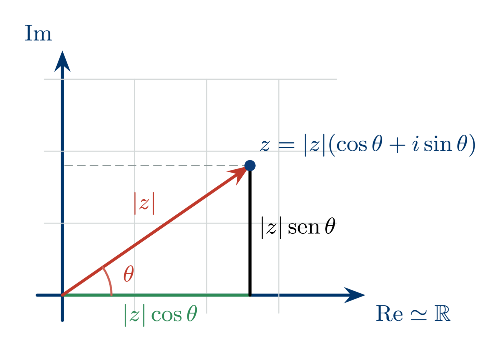
<p><img src="/assets/images/Maths/Analisis/complexpolar.png" alt="complexpolar" /></p>

<p><br /></p>

<h2 id="53-geometric-intuition-of-the-operations-in-mathbbc">5.3. Geometric Intuition of the operations in $\mathbb{C}$.</h2>

<p>In other parts of this same post we asserted that the real numbers were positions on a line, and that this obliges us to interpret the operations of the field with a geometric nuance.</p>

<p>Thus, we stated that in $\mathbb{R}$ the addition was a translation and the product was a homothety. Let's now see how the operations we just defined act in the $Re \times Im$ plane.</p>

<p><br /></p>

<h3 id="531-addition-as-a-torsor">5.3.1. Addition as a torsor.</h3>

<p>In this case, the abelian group $(\mathbb{C},+)$ behaves in $Re \times Im$ making it a <em>torsor</em>. (It is desirable to take a look at the following post to understand the explanation below: <a href="https://gsanmi1.github.io/posts/2026/04/08/VectorSpaces/">vector spaces</a>).</p>

<p>Recapitulating, we know that an affine space is the algebraic structure resulting from using <em>vectors</em> to study a non-empty set in a simply transitive way. Then, a <em>torsor</em> is something prior, more primitive; a torsor is a regular group action of (in this case an abelian) group over a non-empty set, basically an affine space that has forgotten the field's action over the vectors so these can't be scaled and, consequently, you can't scale distances.</p>

<p>We define the pair $(Re \times Im, +)$ being:</p>

\[+ : [Re \times Im] \times (\mathbb{C},+) \to [Re \times Im]\]

\[\quad \quad  \quad (x,y) + z \mapsto (x + z_1, y +z_2)\]

<p><br /></p>

<p>Let's see this is a regular group action:</p>

<ul>
  <li>
    <p>$A1$, taking $0 \in \mathbb{C}$, then: $(x,y) + 0 = (x,y) \quad \forall (x,y) \in Re \times Im$. So there is an identity element.</p>

    <p><br /></p>
  </li>
  <li>
    <p>$A2$, the associativity is immediate from the fact that $(\mathbb{R},+)$ is an abelian group:</p>

\[((x,y) + z)+t = (x+z_1,y+z_2) + t = ([x + z_1] +t_1,[y+z_2]+t_2) =\]

\[(x + [z_1 +t_1],y+[z_2+t_2]) = (x,y) + (z + t)\]

    <p><br /></p>
  </li>
  <li>
    <p><strong>Free</strong> and <strong>Transitivity</strong></p>

    <p>Let's take two points $x,y$ on $Re \times Im$, asking whether $\exists! z \in \mathbb{C} : x + z = y$ is equivalent to ask if the following equation in $\mathbb{R}$, given by the coordinates, has a unique solution:</p>

\[x_i + z_i = y_i \quad i = 1,2\]

    <p>Since $(\mathbb{R},+)$ is an abelian group, we can assert that $z_i = y_i - x_i \in \mathbb{R} \quad i=1,2$ is a solution for each equation and is unique.</p>

    <p>In other words, we have that $\forall P,Q \in Re \times Im \ \exists ! z \in \mathbb{C} : P + z = Q$, so the group action $+$ is also regular and the structure $(Re \times Im, +)$ is a torsor.</p>

    <p><br /></p>
  </li>
</ul>

<p>Intuitively, we can think that any complex $t \in \mathbb{C}$ is a two-dimensional vector $\overrightarrow{t}$, then it can be identified with an arrow over a plane by selecting an origin, in this case; $0 \in \mathbb{C}$. Thus, leveraging the equivalence class of free vectors, doing $z + t$ is, geometrically, as if we take $\overrightarrow{t}$ and translate its base from $0$ to $z$, and then the point referenced by $z + \overrightarrow{t}$ in an affine space and $z+t$ are the same.</p>

<p><img src="/assets/images/Maths/Analisis/complex2.png" alt="complex2" /></p>

<p><br /></p>

<h3 id="532-multiplication-as-a-rotation">5.3.2. Multiplication as a rotation.</h3>

<p>Let's recapitulate and see that we've defined $\mathbb{C}$ as an $\mathbb{R}$-vector space, a two-dimensional vector space, taking $\mathcal{B}:=\Set{e_1 = (1,0), e_2 = (0,1)}$ as the basis; basically we are referring to the fact that $\mathbb{C} = \text{span}(\mathcal{B})$ and any complex $z$ is a linear combination of these two vectors:</p>

\[\forall z \in \mathbb{C} \ \exists \alpha, \beta \in \mathbb{R} : z = \alpha e_1 + \beta e_2\]

<p>This is nothing new and we already worked with this concepts before.</p>

<p><br /></p>

<p>Let's now fix some $w \in \mathbb{C}$ and consider $M_w(z) = wz$, observe that this application is linear, thanks to the commutative and distributive properties of $\mathbb{C}$:</p>

\[M_w(\alpha z_1 + \beta z_2)=w(\alpha z_1 + \beta z_2) =\alpha(wz_1)+\beta(wz_2) = \alpha M_w(z_1) + \beta M_w(z_2)\]

<p>So, as we know, considering $\mathcal{B}$, there exists some $2 \times 2$ matrix that characterizes $M_w$. Take that if $z = (z_x,z_y)_{\mathcal{B}} = z_x + iz_y \in \mathbb{C}$, then:</p>

\[M_w(z) = M_w(z_x + iz_y) = z_xM_w(e_1) + z_yM_w(e_2) = (M_w(1) \ M_w(i)) \begin{pmatrix}z_x \\ z_y\end{pmatrix}\]

<p>So, the columns of our matrix $T$ are where the product with $w$ sends $1$ and $i$, but we can get even further, taking $w = (w_x,w_y)_{\mathcal{B}}$, then:</p>

\[\begin{cases} M_w(1) = (w_x,w_y)(1,0) = (w_x,w_y) \\ M_w(i) = (w_x,w_y)(0,1) = (-w_y,w_x)\end{cases} \implies T_{\mathcal{B}} = (M_w(1) \ M_w(i)) =  \begin{pmatrix}w_x &amp;-w_y \\ w_y &amp; w_x \end{pmatrix}\]

<p><br /></p>

<p>Thus, $M_w(z) = T_{\mathcal{B}}·z = \begin{pmatrix}w_x &amp;-w_y \ w_y &amp; w_x \end{pmatrix}\begin{pmatrix}z_x \ z_y\end{pmatrix} $, but let's be careful for a moment and take a closer look. We do know, from the polar form, that for any complex number $z_x = |z|\cos\theta$ and $z_y = |z|\sin\theta$, meaning:</p>

\[M_w(z) = \begin{pmatrix}w_x &amp;-w_y \\ w_y &amp; w_x \end{pmatrix}\begin{pmatrix}z_x \\ z_y\end{pmatrix} = |w||z| \begin{pmatrix}\cos\theta_w &amp;-\sin\theta_w \\ \sin\theta_w &amp; \cos\theta_w \end{pmatrix}\begin{pmatrix}\cos\theta_z \\ \sin\theta_z\end{pmatrix}\]

<p>Observe that, using trigonometric identities:</p>

\[\begin{pmatrix}\cos\theta_w &amp;-\sin\theta_w \\ \sin\theta_w &amp; \cos\theta_w \end{pmatrix}\begin{pmatrix}\cos\theta_z \\ \sin\theta_z\end{pmatrix} = \begin{pmatrix}\cos\theta_w \cos\theta_z - \sin\theta_w \sin\theta_z \\ \sin\theta_w \cos\theta_z + \cos\theta_w \sin\theta_z \end{pmatrix} = \begin{pmatrix} \cos(\theta_w + \theta_z) \\ \sin(\theta_w + \theta_z) \end{pmatrix}\]

<p>Meaning that, essentially:</p>

\[wz =M_w(z) = |w||z|[\cos(\theta_w + \theta_z) + i · \sin(\theta_w + \theta_z)] = (|w||z|)_{\theta_w + \theta_z}\]

<p>Observe that, to the original $z = |z|(\cos\theta_z + i · \sin\theta_z)$, the product $w·z$ has scaled it by $|w|$ and added the angle $\theta_w$ to $\theta_z$.</p>

<p>Thus the product of complex numbers is basically a homothety centered at $0$ with ratio $|w| \in \mathbb{R}$ composed with a rotation of $\theta_w$ about $0$.</p>

<p><img src="/assets/images/Maths/Analisis/complexrotation.png" alt="complexrotation" /></p>

<p><br /></p>

<h2 id="54-conjugate">5.4. Conjugate.</h2>

<p>The conjugate is one of the most fundamental symmetries in $\mathbb{C}$.  Given $z \in \mathbb{C}$, we define the <em>conjugate</em> of $z$, $\overline{z}$ as the complex number obtained by reflecting it across the real axis, $Re$:</p>

<p><img src="/assets/images/Maths/Analisis/complexconjugate.png" alt="complexconjugate" /></p>

<p>According to the definition we have two equivalent representations. Given: $z \in \mathbb{C}$, then:</p>

\[\overline{z} := \begin{cases} z_x - i z_y \\ |z|_{-\theta_z} \end{cases}\]

<p><br /></p>

<p>The crucial importance of the conjugate is that it captures the invariance for complex solutions to real polynomial equations, this is, if a complex number $z$ is a solution for some real polynomial, then $\overline{z}$ is also a solution.</p>

<p><br /></p>

<h1 id="6-important-properties-of-complex-numbers">6. Important properties of Complex Numbers.</h1>

<p>We have introduced some important notions about complex numbers, let's mix them up in order to present important results about complex numbers:</p>

<p><br /></p>

<h2 id="61-conjugate-properties">6.1. Conjugate properties.</h2>

<p>Let's start by saying that, although an algebraic proof will be provided, most of the properties of the conjugate take place by understanding that the real axis acts as a mirror reflecting what happens on each side of the axis onto the other side.</p>

<p>Thus, the conjugate of the addition is the addition of the conjugates and the conjugate of the product is the product of the conjugate:</p>

<ul>
  <li>
    <p>$\overline{z}+\overline{w}=(z_x - iz_y) + (w_x -iw_y) = (z_x + w_x) - i(z_y+w_y) = \overline{z+w}$</p>
  </li>
  <li>
    <p>$\overline{z} · \overline{w} = |z|_{-\theta_z}|w|_{-\theta_w} = |zw|_{(-\theta_z + - \theta_w)}  = |zw|_{-(\theta_z + \theta_w)} = \overline{z·w}$</p>

    <p><br /></p>
  </li>
</ul>

<p><img src="/assets/images/Maths/Analisis/conjugateaddition.png" alt="conjugateaddition" /></p>

<p><img src="/assets/images/Maths/Analisis/conjugateproduct.png" alt="conjugateproduct" /></p>

<p><br /></p>

<p>Also, observe that adding a complex to its conjugate basically collapses the value onto the real line, so:</p>

<ul>
  <li>$z + \overline{z} = (z_x + z_x) + i(z_y - z_y) = 2Re(z)$</li>
</ul>

<p>And, by the same argument, the subtraction eliminates the real part:</p>

<ul>
  <li>
    <p>$z - \overline{z} = z + - \overline{z} = (z_x - z_x) + i(z_y + z_y) = 2Im(z)$</p>

    <p><br /></p>
  </li>
</ul>

<p><img src="/assets/images/Maths/Analisis/conjugate2.png" alt="conjugate2" /></p>

<p><br /></p>

<p>Also, let's consider $z\overline{z}$, intuitively, we have that we are making over $\overline{z}$ a rotation that negates its own angle, thus it ends up in the positive part of the real axis:</p>

<ul>
  <li>
    <p>$z \neq 0 \implies z\overline{z} \in \mathbb{R}^+$</p>

    <p>Since, $z\overline{z} = |z\overline{z}|_{\theta -\theta} = |z\overline{z}|_0$</p>

    <p><br /></p>

    <p><img src="/assets/images/Maths/Analisis/conjugate3.png" alt="conjugate3" /></p>

    <p><br /></p>

    <p>Lastly, observe also that $z\overline{z} = |z|^2 \implies |z| = \sqrt{z\overline{z}}$.</p>

    <p>Thus $z \in \mathbb{R} \iff z = \overline{z}$</p>

\[|z| = \begin{cases} z \quad z \geq 0 \\ -z \quad z &lt; 0\end{cases}\]

    <p><br /></p>
  </li>
</ul>

<h2 id="62-absolute-value-properties">6.2. Absolute Value properties.</h2>

<p>Note that, we have the following properties of the absolute value:</p>

<ul>
  <li>
    <p>$|z| \geq 0 \wedge (|z| = 0 \iff z = 0)$</p>
  </li>
  <li>
    <p>$|z| = |\overline{z}|$</p>
  </li>
  <li>
    <p>$|zw| = |z| |w|$</p>
  </li>
</ul>

<p>The three properties are immediate as we just see until now.</p>

<ul>
  <li>
    <p>Observe $-1 \leq \cos\theta \leq 1 \iff -|z| \leq |z| \cos\theta \leq |z| \implies | Re(z) | \leq |z|$</p>

    <p><br /></p>
  </li>
</ul>

<p>Lastly, let's consider two points $z,w \in \mathbb{C}$ and consider $z+w$. Then, draft $\triangle(0,z,z+w)$ and observe that the relation between $|z+w|$ and $|z|+|w|$ given by the cosine theorem is:</p>

\[|z+w|^2 = |z|^2 + |w|^2 - 2|z||w|\cos(\pi - (\theta_w - \theta_z)) =|z|^2 + |w|^2 + 2|z||w|\cos(\theta_w - \theta_z)\]

<p>Meaning that $|z+w|$ is $|z|+|w|$ plus an angle correction; let's argue then:</p>

<p>Since, again $|\cos\theta| \leq 1$, then:</p>

\[|z+w|^2 \leq |z|^2 + |w|^2 + 2|z||w| = (|z\| + |w|)^2 \implies |z+w|  \leq |z| + |w|\]

<p>observe that this implication can be asserted since we are always dealing with the square of positive quantities; $|z| \geq 0 \quad \forall z \in \mathbb{C}$</p>

<p><br /></p>

<h2 id="63-cauchy-schwarz-inequality">6.3. Cauchy-Schwarz inequality.</h2>

<h3 id="631-appendix-inner-product-norm-orthogonality">6.3.1. Appendix: Inner product. Norm. Orthogonality.</h3>

<p>Before defining the Cauchy-Schwarz inequality, let's talk a bit about <em>inner products</em>, which are, essentially, the structure that transforms linear algebra into geometry.</p>

<p><br /></p>

<p>We do know, from <a href="https://gsanmi1.github.io/posts/2026/04/08/VectorSpaces/">this post</a>  that vectors from vector spaces are weighted elements from an abelian group through a field's action. They can compound among themselves to generate other vectors and they can be dilated as much as is convenient using the field's scalars, but they can't say much about themselves.</p>

<p>Observe that, through the notion of affine space we acquired a geometric notion about vectors as arrows; the family of all possible vectors emerging from a single origin has vector space structure. Then, intuitively as vectors, these arrows can reference any other arrow in the family and, furthermore, they can also serve as models for other arrows emerging from other points (free vector class) but they can't talk about properties relative to their own relative disposition or what properties remain invariant after a transformation (despite being the subject of these questions) without appealing to geometric statements living in the euclidean space. The only thing that two vectors can say about themselves is whether they are proportional or not, a binary geometrical statement.</p>

<p><br /></p>

<p>This is where the inner product enters; it is the minimal mathematical object that injects this geometric kit onto vector spaces.</p>

<p><br /></p>

<h3 id="632-real-definition-and-conceptual-explanation">6.3.2. Real definition and conceptual explanation.</h3>

<p>Consider $V$ an $\mathbb{R}$-vector space, an <em>inner product</em> over $V$ is an application: $\langle\cdot,\cdot\rangle:V\times V\to\mathbb{R}$, satisfying:</p>

<ul>
  <li>$I1$ <strong>Linearity on first argument</strong>: $\langle x+y,z\rangle = \langle x,z\rangle + \langle y,z\rangle$ and $\langle \alpha x,z\rangle = \alpha\langle x,z\rangle$ such $\alpha \in \mathbb{R}$.</li>
  <li>$I2$ <strong>Symmetry</strong>: $\langle x,y\rangle = \langle y,x\rangle$, observe that this means that the linearity also applies to the second argument, it is <strong>bilinear</strong>.</li>
  <li>$I3$ <strong>Positive definite</strong> $\langle x,x\rangle\geq 0$ and $\langle x,x\rangle = 0 \iff x = 0$</li>
</ul>

<p>Let's observe how a geometric structure distills from these axioms.</p>

<p><br /></p>

<h3 id="633-induced-norm">6.3.3. Induced Norm.</h3>

<p>First, we consider that the root of the inner product of a vector with itself behaves in a special way, we define it as the <em>norm</em> of a vector:</p>

\[\langle x,x \rangle = \|x\|^2\]

<p>Consider two proportional vectors; $x,y \in V: x = \alpha y, \ \alpha \in \mathbb{R}$, from the vector space perspective, $x$ is a deformed version of $y$, then we have that:</p>

\[\langle x,x \rangle = \langle  \alpha y,  \alpha y \rangle = \alpha^2 \langle y,y \rangle \implies  \frac{\|x\|}{\|y\|}= | \alpha |\]

<p>Meaning that the quotient of the norms of two proportional vectors expresses their proportionality factor. Let's consider now:</p>

\[e = \frac{1}{\|x\|}x \implies \|e\| = \frac{\|x\|}{\|x\|}  = 1\]

<p>Thus, we can consider a proportional vector $e$ to $x$ with norm $1$ and say that the norm of any vector expresses the absolute value of the dilation factor relative to a proportional vector of unit norm:</p>

\[x = \alpha ' e \implies \|x\| = |\alpha '| \|e\| = |\alpha '|\]

<p>How amplified or narrowed $x$ is expresses the same information as $e$. And this is what we have agreed to call "magnitude".</p>

<p><br /></p>

<h3 id="634-proper-inner-product-expression">6.3.4. Proper inner product expression.</h3>

<p>Let's now consider $x,y \in V$ non nulls, and consider the norm of $x+y$, then, the inner product $\langle x,y \rangle$ acquires the following form:</p>

\[\|x+y\|^2 = \langle x+y,x+y \rangle = \langle x,x \rangle + \langle y,y \rangle + 2 \langle x,y \rangle = \|x\|^2 + \|y\|^2 + 2\langle x,y \rangle\]

<p>Concluding:</p>

\[\langle x,y \rangle = \frac{1}{2}\big[\|x+y\|^2 - (\|x\|^2 + \|y\|^2)\big]\]

<p>This is, in terms of magnitude, the inner product measures the defect of the squared magnitude of the composition relative to the addition of each individual squared magnitude of the combined vectors.</p>

<p>Let's explain this idea more deeply. Consider the subspace spanned by $x,y$ which is a real subspace of dimension $2$ and isometric to $\mathbb{R}^2$ (in which euclidean geometry applies) and consider some inner product.</p>

<p>Then, select $u,v \in \mathbb{R}^2 : \langle u,v \rangle = 0$ and observe that:</p>

\[\langle u,v \rangle = 0 \iff \|u+v\|^2 = \|u\|^2 + \|v\|^2\]

<p>So, identifying the norm of the vector with its geometric length, by Pythagoras, this is equivalent to asserting that $u \perp v$. The inner product introduces geometry in vector spaces by introducing the notion of <em>disjoint direction</em>; orthogonality is algebraic perpendicularity.</p>

<p>Let's explain it a little more, recapitulating; the inner product gives rise to the norm of a vector which is a quantitative factor of how much it dilates the direction in which the inner product situates it (along with all its proportional vectors). Then, it uses this substratum to understand the relation between the vectors' directions by measuring how much each vector's norm factor contributes to the norm of the combined vector.</p>

<p>If each norm is an expression of its vector's direction, direction interference would affect the norm of the combined vector as the inner product expresses:</p>

\[\|u+v\|^2 = \|u\|^2 + \|v\|^2 + 2 \langle u,v \rangle\]

<p>Identifying the norm with the length in the euclidean plane, perpendicular directions satisfy the Pythagorean theorem as we indicated above. Considering overlapped directions, the same orientation would be expressed as an expansion, $\langle u,v \rangle &gt; 0$, opposite orientation would appear as a retraction $\langle u,v \rangle &lt; 0$ and perpendicular directions will make $\langle u,v \rangle = 0 \iff u \perp v$</p>

<p>It is important to note that what the norm is, is defined by the inner product itself; the geometry inserted (this disjoint notion) depends entirely on how the norm of a vector gets measured, meaning that, depending on the inner product selected, non-perpendicular vectors can still be mathematically orthogonal (extend through disjoint directions) from the product's perspective.</p>

<p><br /></p>

<p>Thus, it is enough to say at this point that $\langle x,y \rangle$ measures how much direction both share or simply how aligned they are in terms of direction and norm.</p>

<p><br /></p>

<h3 id="635-cauchy-schwarz-and-angle-between-two-vectors">6.3.5. Cauchy-Schwarz and angle between two vectors.</h3>

<p>With a basic notion about what inner product is, let's check what Cauchy-Schwarz asserts.</p>

<p><br /></p>

<p>There are two presentations of the same statement, both are mathematically equivalent but admit distinct immediate readings:</p>

<p><br /></p>

<p>Let $x,y \in V$, and $\alpha$ a scalar of the field, then:</p>

\[|\langle x,y \rangle| \leq \|x\| \|y\| \wedge \big(| \langle x,y \rangle| = \|x\| \|y\| \iff \exists \alpha: x = \alpha y \big)\]

<p>According to how we understand the inner product, the Cauchy-Schwarz inequality has a direct meaning; the maximum expression of shared direction is proportionality.</p>

<p>Observe that:</p>

\[x = \alpha y \implies |\langle x,y \rangle| = |\alpha| \langle x,x \rangle = |\alpha| \|x\|\|x\| = \|x\| \|y\|\]

<p><br /></p>

<p>Directly derived from above we have the following expression:</p>

\[\frac{|\langle x,y\rangle|}{\|x\|\,\|y\|} \in [0,1]\]

<p><br /></p>

<p>We finally state that the angle between two vectors is;</p>

\[\theta = \arccos{\frac{|\langle x,y\rangle|}{\|x\|\,\|y\|}}\]

<p><br /></p>

<h2 id="64-rudins-135-theorem">6.4. Rudin's 1.35 theorem.</h2>

<p>Observe that the $1.35$ theorem in Baby Rudin basically takes $\mathbb{C}^n$ as a vector space and an inner product as:</p>

\[\langle x ,y \rangle = \sum_{i=1}^nx_iy_i\]

<p>Then, our previous expression takes the form:</p>

\[|\langle x,y \rangle| \leq \|x\| \|y\| \iff  \left|\sum_{i=1}^nx_iy_i\right| \leq \left|\sum_{i=1}^nx_i \right| \left| \sum_{i=1}^ny_i\right|\]

<p>Let's see now a demonstration. The demonstration is a little tricky, so to speak. The motivation is an orthogonal projection from which denominators have been subtracted. Essentially, the Cauchy-Schwarz inequality asserts the Pythagorean theorem.</p>

<p>Consider $a,b \in \mathbb{C}^n$ and:</p>

\[C = \langle a,b \rangle, \quad B = \langle b,b \rangle = \|b\|^2, \quad A = \|a\|^2\]

<p>Now, let's ask ourselves a question: what is the exact part of $b$ in $a$? Or, in other words, what is that $t$ such that $\langle a -tb,b \rangle = 0$? Check that:</p>

\[\langle a -tb,b \rangle = \langle a,b \rangle - t\langle b,b \rangle = 0 \iff t = \frac{\langle a,b \rangle}{\langle b,b \rangle} = \frac{C}{B}\]

<p>This quotient measures the common direction of $a,b$ in terms of the direction of $b$, or in other words, how much $b$'s magnitude occupies in the shared direction of $a$ with $b$.</p>

<p>Check then, calling $r = a - \frac{C}{B}b$:</p>

\[\langle r,\frac{C}{B}b \rangle = 0 \iff \|r +\frac{C}{B}b\| ^2 = \|a\|^2 = \|r\|^2 + \|\frac{C}{B}b\|^2 = \|r\|^2 + \left|\frac{C}{B} \right|^2\|b\|^2\]

<p>Which means:</p>

\[\|r\|^2 = A - \frac{C^2}{B} \geq 0 \iff A B \geq C^2\]

<p>Now, just changing each part:</p>

\[AB = \|a\|^2\|b\|^2 \geq C^2 = \langle a,b \rangle^2 \implies \|a\| \|b\| \geq |\langle a,b \rangle|\]

<p><br /></p>

<h1 id="7-exercises">7. Exercises.</h1>

<h2 id="71-prove-that-no-order-can-be-defined-in-the-complex-field-that-turns-it-into-an-ordered-field">7.1. Prove that no order can be defined in the complex field that turns it into an ordered field.</h2>

<p>Let's make a brief reminder about what an ordered field is. An ordered field is a field which is also an ordered set and an ordered se which is a non-empty set in which there is defined a binary relation satisfying <em>reflexivity</em>, <em>antisymmetry</em> and <em>trychotomy</em>.</p>

<p>Let's observe a simple fact, given any order $&lt; \subseteq \mathbb{C}^2$, then since $\mathbb{C}$ is a field it satisfies the axiom of the product with the order; this is positive order closure, meaning that the product of any pair of positive numbers should be positive but observe that $i$ simply doesn't fit on it.</p>

<p>It doesnt care how we define it, always this invariance get's transgresed:</p>

<ul>
  <li>
    <p>$i&gt;0 \implies i^2 &gt;0$, but by definition $i^2 = -1 &lt;0$</p>
  </li>
  <li>
    <p>$i&lt; 0 \implies -i&gt;0 \implies (-i) (-i) = i^2 &gt;0$, but again $i^2 = -1 &lt;0$</p>
  </li>
</ul>

<p>Thus, $\mathbb{C}$ can't be an ordered field because $i$ simply don't fit on it.</p>

<p><br /></p>

<p>Let's take a closer look on this fact. The real field is a total ordered set, we discussed that total orders allows to dispose all elements in a sequence along a line. We talk that a representation of this order is the positiveness and negativeness of a number which determines on what side of the $0$ this number lies. Then, we stablished that the multiplication had a geometric nuance as an homothety; in the sense that is an operation with a fixed point from which it dilitates each other point in the set. We defined that an homothety of positive ratio respects the sign and negative ratio reverses it, as a consecuence, any squared number is always positive; if the number it self is positive it stills positive and if not, then his own negativeness make his square positive and this is precisely the rule that $i$ brokes as we saw above.</p>

<p>This is because in $\mathbb{C}$ the product is a homothety combined with a rotation which takes number out of the line, breaking the total order.</p>

<p><br /></p>

<h2 id="72-lexicographic-order">7.2. Lexicographic order.</h2>

<p>Take $z=(a,b),w=(c,d) \in \mathbb{C}$, then we define the <em>lexicographic order</em> as:</p>

\[(a,b) &lt; (c,d) \iff [a &lt; c \vee  (a = c \wedge b &lt; d)]\]

<p>Does $(\mathbb{C}, &lt;)$ have the $LUB$ property?</p>

<p>Let's remember that $LUB$ property stays that for any non-empty upperbounded subset exists the least upperbound element in the universe set.</p>

<p>We can think in the set $A := \Set{z =(a,b) \in \mathbb{C} : a &lt; 1}$, obviously is upperbounded since any $(1,b) \in \mathbb{C}$ is greater than any other element in $A$ so it is upperbounded, but there is not least upper bound, since for any upperbound $(p,q) : p \geq 1$, $(p,q-1)$ is also an upperbound smaller than the first one.</p>

<p><br /></p>

<p>Let's observe that $\mathbb{C}$ is often presented without an order, not only because with the order it can't be an ordered field but also because there even total orders doesn't make it complete.</p>

<p><br /></p>

<h2 id="73-dual-complex-roots">7.3. Dual complex roots.</h2>

<p>Suppose $z = a +bi$, $w = u + iv$ such:</p>

\[a = \left( \frac{|w| + u}{2} \right)^{1/2}, \quad b = \left( \frac{|w| - u}{2} \right)^{1/2}\]

<ol>
  <li>
    <p>Prove that $z^2 = w$ if $v \geq 0$</p>
  </li>
  <li>
    <p>Prove that $\overline{z}^2 = w$ if $v \leq 0$</p>
  </li>
  <li>
    <p>Conclude that every complex number (with one exception!) has two complex square roots.</p>
  </li>
</ol>

<p>First, check that:</p>

\[z^2 = \left( \sqrt{\frac{|w| + u}{2}} + i \sqrt{\frac{|w| - u}{2}} \right)^2 = \frac{|w| + u}{2} - \frac{|w| - u}{2} + 2i \sqrt{\frac{|w| + u}{2} \frac{|w| - u}{2}}\]

\[= u + i\sqrt{|w|^2 - u^2} = u + i\sqrt{(u^2 +v^2) - u^2} = u + i|v| = w\]

<table>
  <tbody>
    <tr>
      <td>Remember that the $n$-th root are defined as a real positive number, $\sqrt[n]{x}\geq 0$, this justifies the absolute value of $</td>
      <td>v</td>
      <td>$ in the computation of $z^2$ and the following result:</td>
    </tr>
  </tbody>
</table>

\[w \in \mathbb{C} : w =(u,v) \neq 0 \implies \exists z \in \mathbb{C}: w = \begin{cases} z^2 \quad v \geq 0 \\ \overline{z}^2 \quad v \leq 0 \end{cases}\]

<p><br /></p>

<h2 id="74-if-z-is-a-complex-number-prove-that-there-exists-an-r--0-and-a-complex-number-w-with-w--1--z-rw-are-w-and-r-always-uniquely-determined-by-z">7.4. If $z$ is a complex number, prove that there exists an $r &gt; 0$ and a complex number $w$ with $|w| = 1 : z= rw$. Are $w$ and $r$ always uniquely determined by $z$?</h2>

<p>Take the polar form of $z$ and call:</p>

\[z = |z|_{\theta} = |z|(\cos\theta + i\sin\theta) \implies \begin{cases} r = |z| \\ w =\cos\theta + i\sin\theta \end{cases}\]

<p>Observe that; $r\geq 0$,  $|w| = \sqrt{cos^2\theta + sin^2\theta} = \sqrt{1} = 1$ and $z = rw$. Observe also that to compute both elements $z$ is only needed, so both are uniquely determined by $z$.</p>

<p><br /></p>

<h2 id="75-generalization-of-the-triangle-inequality">7.5. Generalization of the triangle inequality.</h2>

<p>If $z_1,…,z_n \in \mathbb{C}$, prove that:</p>

\[\left|\sum_{i=1}^n z_i \right| \leq \sum_{i=1}^n |z_i|\]

<p><br /></p>

<p>Let's proof this result by induction.</p>

<ul>
  <li>
    <p>First, for $n=2$, if we take $z_1,z_2 \in \mathbb{C}$, then, the real inner product given by the absolute value of a complex number states that:</p>

\[|z_1 + z_2|^2 = |z_1|^2 + |z_2|^2 + 2\langle z_1,z_2 \rangle \leq |z_1|^2 + |z_2|^2 + 2|\langle z_1,z_2 \rangle|\]

    <p>And by Cauchy-Schwarz is:</p>

\[|z_1|^2 + |z_2|^2 + 2|\langle z_1,z_2 \rangle|\leq |z_1|^2 + |z_2|^2 + 2 |z_1||z_2| = (|z_1| + |z_2|)^2\]

    <p>Thus, since the absolute value is always non-negative :</p>

\[|z_1 + z_2|^2 \leq (|z_1| + |z_2|)^2 \iff |z_1 + z_2| \leq |z_1| + |z_2|\]

    <p>And we prove the result for $n=2$.</p>

    <p><br /></p>
  </li>
  <li>
    <p>Let's consider it true for some $n$. Consider $z_1,…,z_n \in \mathbb{C}$, $w = \sum_{i=1}^n z_i$ and some $z \in \mathbb{C}$, then:</p>

\[|z_1 \cdots + z_n + z| = |w + z| \leq |w| + |z| = |z_1 \cdots + z_n | + |z| \leq |z_1|  \cdots + |z_n| + |z|\]

    <p><br /></p>
  </li>
</ul>

<h2 id="76-if-xy-in-mathbbc-prove-that">7.6. If $x,y \in \mathbb{C}$, prove that:</h2>

\[||x| - |y|| \leq |x - y|\]

<ul>
  <li>
    <p>First, take $|x| = |x -y + y| \leq |x -y| + |y| \iff |x| - |y| \leq |x-y|$.</p>
  </li>
  <li>
    <p>Second $|y| = |y-x + x| \leq |y - x| + |x| \iff |y| - |x| = - (|x| - |y|) \leq |y -x| = |x - y|$</p>
  </li>
</ul>

<p>Ultimately:</p>

\[-|x - y| \leq |x| - |y| \leq |x-y| \iff ||x| - |y|| \leq |x - y|\]]]></content><author><name>German Sanmi</name></author><category term="Maths" /><category term="analisis_rudin" /><category term="Maths" /><summary type="html"><![CDATA[0. Index]]></summary></entry><entry xml:lang="en"><title type="html">2. Introduction to VectorSpaces</title><link href="/posts/2026/04/08/VectorSpaces/" rel="alternate" type="text/html" title="2. Introduction to VectorSpaces" /><published>2026-04-08T09:00:00+00:00</published><updated>2026-04-08T09:00:00+00:00</updated><id>/posts/2026/04/08/VectorSpaces</id><content type="html" xml:base="/posts/2026/04/08/VectorSpaces/"><![CDATA[<ol>
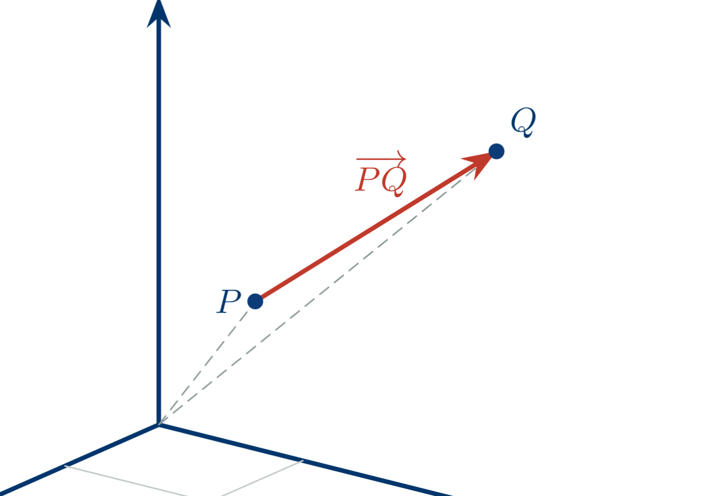
  <li>Conceptual Approach: Algebra and Algebraic Structures.
    <ul>
      <li>1.1. Algebra as a discipline.</li>
      <li>1.2. Algebraic Structures.
        <ul>
          <li>1.2.1. One operation algebraic structures.</li>
          <li>1.2.2. Two operations algebraic structures.</li>
        </ul>
      </li>
    </ul>
  </li>
  <li>Vector spaces.
    <ul>
      <li>2.1. Actions. Algebraic Actions.
        <ul>
          <li>2.1.1. Definition.</li>
          <li>2.1.2. Group's Action.</li>
        </ul>
      </li>
      <li>2.2. Field's action. Vector Space.
        <ul>
          <li>2.2.1. Definition.</li>
          <li>2.2.2. Conceptually Approach.</li>
        </ul>
      </li>
      <li>2.3. Examples.
        <ul>
          <li>2.3.1. The n-tuple space.</li>
          <li>2.3.2. The space of m x n matrices.</li>
          <li>2.3.3. The space of functions from a set to a field.</li>
          <li>2.3.4. The space of polynomial functions over a field K.
            <ul>
              <li>2.3.4.1. Introduction to polynomials.</li>
              <li>2.3.4.2. Vector space of the polynomial functions over a field K.</li>
            </ul>
          </li>
        </ul>
      </li>
      <li>2.4. Immediate Properties from vector spaces.</li>
    </ul>
  </li>
  <li>Vector Spaces and Geometry.
    <ul>
      <li>3.1. Analytic Geometry: The affine space.
        <ul>
          <li>3.1.1. Definition.</li>
          <li>3.1.2. Isomorphism by origin.</li>
        </ul>
      </li>
      <li>3.2. Vectors as geometric objects: Arrows.
        <ul>
          <li>3.2.1. Bound arrows. Vectors as arrows.</li>
          <li>3.2.2. Equipolence class: Free vectors.
            <ul>
              <li>3.2.2.1. Appendix: Equivalence Class.</li>
              <li>3.2.2.2. Vector equipolence.</li>
            </ul>
          </li>
        </ul>
      </li>
    </ul>
  </li>
  <li>Summary.</li>
</ol>

<h1 id="1-conceptual-approach-algebra-algebraic-structures">1. Conceptual Approach. Algebra, Algebraic Structures.</h1>

<h2 id="11-algebra-as-a-discipline">1.1. Algebra as a discipline.</h2>

<p>Let's start by introducing what <strong>Algebra</strong> is. Algebra is the mathematical discipline in charge of the study of what <em>operating with the elements of a set means</em>: how items of a set are combined through an operation and what properties emerge from that context. It doesn't study the elements (like arithmetic would do) but the properties of the operations between them.</p>

<p><br /></p>

<h2 id="12-algebraic-structures">1.2. Algebraic Structures.</h2>

<p>An <strong>algebraic structure</strong> is a set $(S, \Omega)$ where:</p>

<ul>
  <li>$S \neq \varnothing$</li>
  <li>$\Omega$ is a collection of operations over $S$ (and maybe other sets as we will see) along with a sequence of rules called <em>axioms</em> that these operations satisfy.</li>
</ul>

<p>This is the minimal basic item of study in algebra; a finite number of operations over a set defined by axioms. Our task is to comprehend how these operations behave through the axioms, applying classical logic.</p>

<p>In the previous section we already provided an introduction to algebraic structures through the number sets and then introduced a solid idea of the group and then the field. Our objective was to present a formalization about linear equations over a field.</p>

<p>We can review and develop the ideas presented in the <a href="https://gsanmi1.github.io/posts/2026/02/06/Linear_Equations/">Linear Equation section</a> to understand the natural progression and the algebraic structures towards the vector space.</p>

<p><br /></p>

<h3 id="121-one-operation-algebraic-structures">1.2.1. One operation algebraic structures.</h3>

<p>Let $G := (S, \Omega) : \Omega := \Set{\star}$, where $\star : S \times S \to S$ is an internal operation (a function).</p>

<p>Then we define:</p>

<ul>
  <li>
    <p>$G$ (or $S$ by default) is said to be a <em>Magma</em> if $\star$ only verifies the closure property:</p>

    <ul>
      <li>$a \star b \in S \ \ \forall a,b \in S$ (Closure)</li>
    </ul>

    <p>Observe that this structure is the minimal one, and his only property is forced by $\star$ definition.</p>

    <p><br /></p>
  </li>
  <li>
    <p>$G$ is a <em>semigroup</em> if it also verifies associativity:</p>

    <ul>
      <li>$a \star b \in S \ \ \forall a,b \in S$ (Closure)</li>
      <li>$(a \star b) \star c = a \star (b \star c) \ \ \forall a,b \in S$ (Associativity)</li>
    </ul>

    <p><br /></p>
  </li>
  <li>
    <p>A <em>monoid</em> is a semigroup that also has the identity element $e \in S$ relative to $\star$ verifying:</p>

    <ul>
      <li>$a \star b \in S \ \ \forall a,b \in S$ (Closure)</li>
      <li>$(a \star b) \star c = a \star (b \star c) \ \ \forall a,b \in S$ (Associativity)</li>
      <li>$ \exists e \in S \ \ \forall a \in S : e \star a = a \star e = a$ (Identity)</li>
    </ul>

    <p><br /></p>
  </li>
  <li>
    <p>Now we enter the comfort zone; a <em>Group</em> is a monoid which verifies the existence of an inverse for each item in $S$:</p>

    <ul>
      <li>$a \star b \in S \ \ \forall a,b \in S$ (Closure)</li>
      <li>$(a \star b) \star c = a \star (b \star c) \ \ \forall a,b,c \in S$ (Associativity)</li>
      <li>$ \exists e \in S \ \ \forall a \in S : e \star a = a \star e = a$ (Identity)</li>
      <li>$\forall a \in S \ \ \exists a' \in S : a \star a' = a' \star a = e$ (Inverse)</li>
    </ul>

    <p><br /></p>
  </li>
</ul>

<p>Let's observe that each axiom lets us do something new in the structure; each new rule is a new capability based on the defining of invariants along the structure;</p>

<ul>
  <li>
    <p>The closure guarantees internal compositions; the belonging of any composition to $S$ remains constant.</p>
  </li>
  <li>
    <p>The associativity guarantees order-independence as long as the direction in the composition remains the same, meaning that $(a\star b) \star c$ and $a\star (b \star c)$ are the same object in the sense that we can talk about $a\star b \star c$ to refer to any of them, no matter what you compose first.</p>
  </li>
  <li>
    <p>The existence of the identity guarantees the existence of a way to operate that does nothing, concreted in an element of $S$ called the identity. The composition of $e$ with any item of $S$ in any direction remains constant and is the very same item.</p>
  </li>
  <li>
    <p>The existence of the inverse makes use of the identity to guarantee a way to operate that lets you reverse the operation. The composition of any item with its inverse in any direction remains constant and is the identity.</p>
  </li>
</ul>

<p><br /></p>

<p>Observe that these are the main invariants in operations because these are the smallest subset of rules that allow you to define constraints about some elements (equations) and comfortably operate to isolate them in order to fully understand what that constraint is equivalent to and what a valid item is.</p>

<p>Suppose there is an interest in finding the relation between two elements $a,b \in S$, this is, $b$ is the composition of $a$ with some other element $x \in S$ which we are going to call the <em>unknown</em>: $a \star x = b$. Now, let's observe:</p>

\[a^{-1} \star (a \star x) = a^{-1} \star b\]

<p>Step by step, the closure axiom asserts that $a^{-1} \star (a \star x) = a^{-1} \star b \in S$ and the proposal makes sense; the associativity establishes that $a^{-1} \star (a \star x)  = a^{-1} \star a \star x= (a^{-1} \star a) \star x$, or that we can choose the order of the composition as we please. Then, the identity and the inverse cooperate together to simplify the expression; the inverse makes $a$ disappear, it substitutes it for the identity and the identity composed with any other item is that other item, thus:</p>

\[a^{-1} \star (a \star x) = (a^{-1} \star a) \star x = e \star x = x = a^{-1} \star b\]

<p>These four invariants are summarized in the idea of <em>group</em>.</p>

<p>This idea of group can be extended by introducing the <em>commutativity</em> which defines the composition under direction as an invariant:</p>

\[a \star b = b \star a \ \ \forall a,b \in S\]

<p>This allows reorganizing, making the simplification of expressions even more comfortable.</p>

<p><br /></p>

<h3 id="122-two-operations-algebraic-structures">1.2.2. Two operations algebraic structures.</h3>

<p>Until now, we've defined an algebraic structure that contemplates only one operation; let's now introduce algebraic structures with two operations.</p>

<p><br /></p>

<p><strong>Rings</strong></p>

<p>First, the rings; a ring is a triple $(K,+,\ ·)$ such:</p>

<ul>
  <li>$(K,+)$ is a group and introduces the four properties seen above.</li>
  <li>$(K, \ ·)$ is a monoid, it drops the existence of the inverse for any element of $R$.</li>
  <li>
    <p>$+$ and $·$ relates themselves by the distributive law:</p>

\[a(b+c) = ab + ac \wedge (b+c)a = ba + ca\]

    <p>We say both operations are compatible.</p>

    <p><br /></p>
  </li>
</ul>

<p>The ring introduces the second operation in a soft way; hanging on the existence of the inverse allows it to fit in many well-studied structures such:</p>

<ul>
  <li>
    <p><strong>Integers ring</strong>; $(\mathbb{Z},+, \ ·)$, where for example $\forall a ( a \in \mathbb{Z} \wedge a \neq \pm 1 \implies a^{-1} \notin \mathbb{Z})$.</p>

    <p><br /></p>
  </li>
  <li>
    <p><strong>Polynomial ring</strong>; with coefficients in a field $F$; $F[x]$ is a ring 
but not a field. For instance, $x$ has no multiplicative inverse:</p>

    <p>$\forall q \in F[x] \setminus {0} \ \deg(x \cdot q) = 1 + \deg(q) \geq 1 \neq 0 = \deg(1)$</p>

    <p>So the equation $x \cdot q = 1$ has no solution in $F[x]$</p>

    <p><br /></p>
  </li>
  <li>
    <p><strong>Matrix ring</strong>; we've already seen that $(M_n(F)\setminus 0, \ ·)$ has no inverse for every element of $M_n(F)$; remember that we already saw that not every matrix is invertible, only those row-equivalent to the identity $I_n$</p>

    <p><br /></p>
  </li>
</ul>

<p>The mathematical world is full of structures with two operations where division fails.</p>

<p><br /></p>

<p><strong>Field</strong></p>

<p>Then the concept of the field can be thought as an extension of the ring where each element has an inverse for the product operation except the zero element.</p>

<p>However, we want to present another perspective of a field.</p>

<p>Above we built step by step from the smallest algebraic structure <em>Magma</em> to the <em>Group</em> and his four axioms and we conclude the importance of such structure was that it allows to present and solve equations:</p>

\[a \star x = b \iff x = a^{-1} \star b\]

<p>Then, the field $K$ aims to extend the same idea for two operations departing from the group structure. This means that a field is a triple $(K,+, \ ·)$ such:</p>

<ul>
  <li>$(K, +)$ is an abelian group.</li>
  <li>$(K \setminus \Set{0}, \ ·)$ is an abelian group.</li>
  <li>$+$ and $·$ are compatible.</li>
  <li>$1 \neq 0$</li>
</ul>

<p>This basically means that the field intends to be the structure in which equations can be defined and solved in two operations simultaneously; the motivation was to build an algebraic framework for common arithmetic operations in $\mathbb{R}, \mathbb{Q},…$ and other common fields.</p>

<p><br /></p>

<h1 id="2-vector-spaces">2. Vector spaces.</h1>

<p>Before, we've seen a set of axioms that rule how a set of operations $\Omega$ behaves in a non-empty set $K$. We extend this concept to two sets $(K,V)$ where $K$ is a field and $V$ is a group and both are related by a field-action.</p>

<p>Let's dive into this.</p>

<p><br /></p>

<h2 id="21-actions-algebraic-actions">2.1. Actions. Algebraic Actions.</h2>

<h3 id="211-definition">2.1.1. Definition.</h3>

<p>First, let's define what an action is. Let $A$ and $S$ be two sets, then we define an action as a function:</p>

<p>\(\varphi: A \times S \to S\)
\(\ \ \ \ \ \ \ (a,s) \to s\)</p>

<p>It grabs two elements, one from $A$ and another from $S$ and it maps it to a third element from $S$.</p>

<p>As defined, this function doesn't have any interest at all; it becomes interesting when $\varphi$ respects the structure of $A$; this way it is said that an action transforms $S$ using $A$'s algebraic structure.</p>

<p><br /></p>

<h3 id="212-groups-action">2.1.2. Group's Action.</h3>

<p><strong>Group's action</strong></p>

<p>Consider again $(G,S,\varphi)$ such that $\varphi : G \times S \to S$, let's suppose now that $G$ is a group for some internal operation $\star : G \times G \to G$.</p>

<p>In this context, we impose two rules $A1$, $A2$ over $\varphi : A \times S \to S$. In total, the triple $(G,S,\varphi)$ satisfies:</p>

<ul>
  <li>
    <p><strong>Closure</strong>: $\varphi(a,s) \in S \ \ \forall a \in G, s \in S$, forced by $\varphi$ definition.</p>

    <p><br /></p>
  </li>
  <li>
    <p><strong>(A1) Identity</strong>: Be $e \in G$ the identity on $G$ then we require: $\varphi(e,s) = s \ \ \forall s \in S$</p>

    <p>Meaning that the $G$'s identity doesn't move anything through $\varphi$.</p>

    <p><br /></p>
  </li>
  <li>
    <p><strong>(A2) Associativity</strong>: $\varphi(a,\varphi(b,s)) = \varphi(a \star b,s) \ \ \forall a,b \in G, s \in S$</p>

    <p>Observe that this resembles the order invariant we talked about in groups; as long as the direction of the composition remains still ($a \to b \to s$) it doesn't matter the order in which you perform these compositions.</p>

    <p>Composing $b$ with $s$ through $\varphi$ and then this with $a$ is the same that "multiply" $a \star b$ in $G$ and then compose it with $s$ through $\varphi$. Check that if we write $a \star b = ab \wedge \varphi(a,s) = a\ ·s$ then, the rule above states that:</p>

\[a \ ·(b \ ·s) = (ab)\ ·s \ \ \forall a,b \in G, s \in S\]

    <p>And it appears more familiar.</p>

    <p><br /></p>
  </li>
  <li>
    <p><strong>Inverse</strong>: Observe this is not labeled as an axiom because it can be deduced from the two above but is included from pedagogic reasons.</p>

    <p>The idea of the inverse on a group intends to formalice the idea of revert a composition or go back. Thus, we are looking to demonstrate that, calling $\varphi_a(s) = \varphi(a,s)$</p>

\[\forall \varphi_a \ \exists \varphi^{-1}_{a}  \ \forall s \in S: \varphi_a(\varphi^{-1}_{a}(s)) = \varphi^{-1}_{a}(\varphi_a(s)) = s\]

    <p>Let's take $x = a^{-1}$ and observe that applying $A2$, $A1$ and the existence of the inverse in $G$ we get:</p>

\[a^{-1} \ ·(a \ · s) = (a^{-1}a) \ · s = e \ · s = s\]

\[a \ · (a^{-1} \ · s) = (aa^{-1}) \ · s = s\]

    <p>Meaning that $\varphi^{-1}_{a}= \varphi_{a^{-1}} \ \ \forall a \in G$.</p>

    <p><br /></p>
  </li>
</ul>

<p>Thus, this four properties makes that the triple $(G,S,\varphi)$ behaves like a group in the sense that we can define and solve equations over the elements of $S$ which remember, initially wasn't a group:</p>

\[\varphi_a(x) = s \iff x = \varphi_{a^{-1}}(s)\]

<p>Meaning that we can treat the elements of $S$ as elements over which we can define constraints, relations, etc.</p>

<p>Although, it is worth remembering that $S$ is not a group and neither is the triple $(G,S, \varphi)$; what $S$ has acquired through $\varphi$ is a family of reversible parametrized transformations by the group $G$. It is a way to use $G$ in order to study $S$.</p>

<p><br /></p>

<h2 id="22-fields-action-vector-space">2.2. Field's action. Vector Space.</h2>

<h3 id="221-definition">2.2.1. Definition.</h3>

<p>Now consider again a triple $(K,V,\ ·)$, where $K$ is a field and $V$ is an abelian group and $·: K \times V \to V$ is a field's action.</p>

<p>As we said before this action respects the algebraic structure of $K$, which remember; is a combined abelian group over two different compatible operations, by forcing the following axioms:</p>

<ul>
  <li><strong>M1</strong>: $1_K \ · v = v$. The identity over the product doesn't transform anything.</li>
  <li><strong>M2</strong>: $\alpha \ · (\beta \ · v) = (\alpha \beta) \ · v \ \ \forall \alpha, \beta \in K, v \in V $. associativity resemblance, order-independence while direction stays still.</li>
  <li><strong>D1</strong>: $\alpha \ · (u + v) = \alpha \ · u + \alpha \ · v \ \ \forall \alpha \in K, u, v \in V $. Compatibility between $·$ and $+$ in $V$.</li>
  <li><strong>D2</strong>: $(\alpha + \beta) \ · v =\alpha \ · v + \beta \ · v \ \ \forall \alpha, \beta \in K, v \in V$. Compatibility between $·$ and $+$ in $K$.</li>
</ul>

<p>This four axioms plus the four axioms of the group $V$ gives us the eight axioms of the vector space $(K,V, \ ·)$.</p>

<p><br /></p>

<h3 id="222-conceptually-approach">2.2.2. Conceptually Approach.</h3>

<p>This time, a field's action over a group doesn't intend to give an algebraic structure to $V$; instead it provides, through $K$, a uniform deformation mechanism. The arithmetic system of $K$ as a field is used to perform richer algebraic manipulations on $V$ as a group.</p>

<p>$·: K \times V \to V$ gives to $V$ a parametric scaling mechanism through $(K,+, \ ·)$ which, ultimately, allows a coherent way to perform linear combinations on the elements of $V$.</p>

<p>Let's dive into "scaling", "linear" and "linear combination" terms in order to understand what this introduction means.</p>

<p><br /></p>

<p><strong>Scaling.</strong></p>

<p>Scaling is about relating $V$'s elements using $K$'s elements as mediators. The term "scalar" comes from scale; changing the size without changing the essential nature of the object.</p>

<p>Then, being $u,v \in V$ and $\alpha \in K : \alpha \neq 0$, when we say that $u = \alpha \ · v$, we are really saying $u$ is obtained from $v$, keeping its structural information since, thanks to $K$ being a field and $·$ respecting $K$'s properties, we can revert this operation and go back from $u$ to $v$. Let's see that by $M2$ and $M1$ we can guarantee the existence of some $\beta \in K$ such that $\beta \ · u = v$. Take $\beta = \alpha ^{-1}$ and:</p>

\[\alpha^{-1} \ · u = \alpha^{-1} \ · (\alpha \ · v) \underbrace{=}_{M2} (\alpha^{-1} \alpha) \ · v = (1_K) \ · v \underbrace{=}_{M1}  v\]

<p>In this context we say that $u$ and $v$ are <em>proportional</em>. Specifically, there exists an entire family of elements to which $u$ is proportional: $\Set{\alpha v : \alpha \in K \wedge \alpha \neq 0} \subseteq V$.</p>

<p><br /></p>

<p><strong>Linear &amp; Linear Combinations.</strong></p>

<p>Linear refers to independent contributions of several parts which do not interfere between them.</p>

<p>In this case, a linear combination is the minimal operation that takes place in the triple $(K,V, \ ·)$; independent contribution of proportional components of $V$.</p>

<p>Is the most general way to combine while respecting the principle of independent contributions:</p>

\[\alpha v + \beta u: \alpha , \beta \in K \ \ u, v \in V\]

<p>Observe that $D1$ and $D2$ guarantee that $K$ and $V$ respect this object on $(K,V,\ ·)$.</p>

<p><br /></p>

<p><strong>Vector Space</strong></p>

<p>Thus, $(K,V, \ ·)$ is the algebraic environment where a set of objects can be combined by independent contributions weighted by a field. A field's action is the mechanism that imports the arithmetic of $K$ as a system of intensities applicable to the elements of $V$.</p>

<p>A vector space is nothing but, conceptually, a functional linear combination system and his elements are called vectors.</p>

<p><br /></p>

<p><strong>Vectors</strong></p>

<p>Thus, vectors are elements of an algebraic structure called vector space whose elements relate through linear combinations verifying the eight axioms presented before.</p>

<p>Being the vector space an algebraic structure means that vectors (and vector spaces) are nothing; as we said at the start of these very notes, algebra cares about how to operate and the properties that emerge from some defined operable structure.</p>

<p>In other words; vectors are the elements of an abelian group $V$ on which a field $K$ acts through a "deformation" mechanism. This action, the combination or composition of these deformed elements of $V$, is what we call linear combinations: weighted sums where each element of $V$ contributes with an intensity set by $K$.</p>

<p>The corollary from this assertion is that what really matters is that there are objects (matrices, polynomials, arrows, etc.) that, with the right operations, verify the vector space axioms; thus, they are vectors and all the machinery defined around them works also for these objects.</p>

<p><br /></p>

<h2 id="23-examples">2.3. Examples.</h2>

<p>Let's see a few mathematical objects that algebraically behave as vector spaces.</p>

<h3 id="231-the-n-tuple-space">2.3.1. The n-tuple space.</h3>

<p>Consider $F$ a field, then the algebraic structure $(F^n,+)$ with the addition behaving as:</p>

\[+: F^n \times F^n \to F^n \mid x + y := \begin{pmatrix}x_1 + y_1\\ \vdots \\ x_n+y_n\end{pmatrix} \in F^n\]

<p>Observe that the properties of the abelian group $(F,+)$ expand to $(F^n,+)$ so this is also an abelian group.</p>

<p>Thus, defining the function defined as:</p>

<p>\(· : F \times F^n \to F^n\)
\((\alpha, \begin{pmatrix}x_1 \\ \vdots \\ x_n\end{pmatrix} ) \to  \begin{pmatrix}\alpha x_1 \\ \vdots \\ \alpha x_n\end{pmatrix}\)</p>

<p>Verifies the field's action axioms:</p>

<ul>
  <li>
    <p><strong>M1</strong>: $1 \ · \begin{pmatrix}x_1 \ \vdots \ x_n\end{pmatrix} = \begin{pmatrix}1x_1 \ \vdots \ 1x_n\end{pmatrix} = \begin{pmatrix}x_1 \ \vdots \ x_n\end{pmatrix} \ \ \forall x \in F^n$</p>

    <p><br /></p>
  </li>
  <li>
    <p><strong>M2</strong>: $\alpha \ ·( \beta \ · \begin{pmatrix}x_1 \ \vdots \ x_n\end{pmatrix}) = \alpha \ · \begin{pmatrix}\beta x_1 \ \vdots \\beta x_n\end{pmatrix} = \begin{pmatrix}\alpha \beta x_1 \ \vdots \\alpha \beta x_n\end{pmatrix} = (\alpha \beta) \ · \begin{pmatrix}x_1 \ \vdots \ x_n\end{pmatrix} \ \ \forall \alpha, \beta \in F, x \in F^n$</p>

    <p><br /></p>
  </li>
  <li>
    <p><strong>D1</strong>:</p>

\[\alpha \ · (\begin{pmatrix}x_1 \\ \vdots \\ x_n\end{pmatrix} + \begin{pmatrix}y_1 \\ \vdots \\ y_n\end{pmatrix}) = \alpha \ · \begin{pmatrix}x_1 +y_1 \\ \vdots \\ x_n + y_n\end{pmatrix} = \begin{pmatrix}\alpha (x_1 + y_1) \\ \vdots \\ \alpha (x_n + y_n)\end{pmatrix} = \begin{pmatrix}\alpha x_1 + \alpha y_1\\ \vdots \\ \alpha x_n + \alpha y_n\end{pmatrix}\]

\[= \begin{pmatrix}\alpha x_1 \\ \vdots \\ \alpha x_n\end{pmatrix} + \begin{pmatrix}\alpha y_1 \\ \vdots \\ \alpha y_n\end{pmatrix} = \alpha \ · \begin{pmatrix}x_1 \\ \vdots \\ x_n\end{pmatrix} + \alpha \ · \begin{pmatrix}y_1 \\ \vdots \\ y_n\end{pmatrix} \ \ \forall x,y \in F^n, \alpha \in F\]

    <p><br /></p>
  </li>
  <li>
    <p><strong>D2</strong>:</p>

\[(\alpha + \beta)\ · \begin{pmatrix}x_1 \\ \vdots \\ x_n\end{pmatrix} = \begin{pmatrix}(\alpha + \beta)x_1 \\ \vdots \\ (\alpha + \beta)x_n\end{pmatrix} = \begin{pmatrix}\alpha x_1 + \beta x_1 \\ \vdots \\ \alpha x_n + \beta x_n\end{pmatrix} = \begin{pmatrix}\alpha x_1 \\ \vdots \\ \alpha x_n\end{pmatrix} + \begin{pmatrix}\beta x_1 \\ \vdots \\ \beta x_n\end{pmatrix}\]

\[= \alpha \ · \begin{pmatrix}x_1 \\ \vdots \\ x_n\end{pmatrix} + \beta \ · \begin{pmatrix}x_1 \\ \vdots \\ x_n\end{pmatrix}\]

    <p><br /></p>
  </li>
</ul>

<p>Thus, the triple $\big(F,(F^n,+), \ · \big)$ satisfies:</p>

<ul>
  <li>$F$ being a field.</li>
  <li>$(F^n,+)$ an abelian group.</li>
  <li>$(\ ·)$ is a field's action (an action satisfying $M1,M2,D1,D2$ axioms).</li>
</ul>

<p>And is a vector space.</p>

<p>Observe that, as a special case, $(\mathbb{R},(\mathbb{C}^n,+), \ ·)$ is a vector space.</p>

<p><br /></p>

<h3 id="232-the-space-of-m-x-n-matrices">2.3.2. The space of m x n matrices.</h3>

<p>Let's consider the set $M_{m \times n}(F) = F^{m \times n}$ with</p>

\[+: F^{m \times n} \times F^{m \times n} \to F^{m \times n}\]

\[(a_{ij}) + (b_{ij}) := \big((a_{ij} + b_{ij})_{ij} \big)\in F^{m \times n}\]

<p>Observe that again addition in $F^{m \times n}$ is extended from $(F,+)$ which is an abelian group so $(F^{m \times n},+)$ is also an abelian group, the argument is the same, addition in $F^{m \times n}$ are $mn$ additions on $F$.</p>

<p><br /></p>

<p>Also, consider the action:</p>

<p>\(· : F \times F^{m \times n} \to F^{m \times n}\)
\((\alpha, (a_{ij}) ) \mapsto  (\alpha a_{ij})\)</p>

<p>Observe that:</p>

<ul>
  <li>
    <p><strong>M1</strong>: $1 \ · (a_{ij}) = (1 a_{ij}) = (a_{ij}) \ \ \forall (a_{ij}) \in F^{m \times n}$</p>

    <p><br /></p>
  </li>
  <li>
    <p><strong>M2</strong>: $\alpha \ · (\beta \ · (a_{ij})) = \alpha \ · (\beta (a_{ij})) = (\alpha \beta (a_{ij})) = (\alpha \beta) \ · (a_{ij}) \ \ \forall \alpha, \beta \in F, (a_{ij}) \in F^{m \times n}$</p>

    <p><br /></p>
  </li>
  <li>
    <p><strong>D1</strong>: \(\alpha \ · ((a_{ij}) + (b_{ij})) = \alpha \ · \big((a_{ij} + b_{ij})_{ij} \big) = \big(\alpha (a_{ij} + b_{ij})_{ij} \big) = \big(((\alpha a_{ij}) + (\alpha b_{ij}))_{ij} \big)\)</p>

\[= (\alpha a_{ij}) + (\alpha b_{ij}) = \alpha \ · (a_{ij}) + \alpha \ · (b_{ij}) \ \ \forall \alpha \in F, (a_{ij}),(b_{ij}) \in F^{m \times n}\]

    <p><br /></p>
  </li>
  <li>
    <p><strong>D2</strong>:</p>

\[(\alpha + \beta) \ · (a_{ij}) = (((\alpha + \beta)a_{ij})_{ij}) = ((\alpha a_{ij} + \beta a_{ij})_{ij}) = (\alpha a_{ij}) + (\beta a_{ij}) \ \ \forall \alpha, \beta \in F, (a_{ij})\in F^{m \times n}\]

    <p><br /></p>
  </li>
</ul>

<p>This way, $F$ is a field, $(F^{m \times n},+)$ is an abelian group and $( \ ·)$ is a field's action of $F$ over $(F^{m \times n},+)$.</p>

<p>Thus, $\big(F,(F^{m\times n},+), \ · \big)$ is a vector space.</p>

<p><br /></p>

<p>Let's observe that, despite we already touched some operation properties from the addition and product of matrix, the fact that this set is a vector space finish refining the details of both operations and how they related them selves.</p>

<p><br /></p>

<h3 id="233-the-space-of-functions-from-a-set-to-a-field">2.3.3. The space of functions from a set to a field.</h3>

<p>Consider now some field $K$ and some set $S \neq \varnothing$, then, remember that being $f : S \to K$ a function, this gets identified with its graph $f \subseteq S \times K : (\forall s \in S \ \exists ! \alpha \in K \mid (s,\alpha) \in f)$, meaning that a function is a relation in which every element of the domain has a unique image through $f$.</p>

<p>Then, the set of all the relations from $S$ to $K$ that are applications is:</p>

\[K^S := \Set{f \in \mathcal{P}(S \times K) \mid \forall s \in S \ \exists ! \alpha \in K : (s,\alpha) \in f}\]

<p>In this context, we agree on the notation  $f(s) = \alpha \iff (s,\alpha) \in f$, then let's call:</p>

\[f = \Set{(s,f(s)) \mid s \in S}\]

<p>This is the set of all the functions from $S$ to $K$ and define an addition over $K^S$ elements as:</p>

\[+ : K^S  \times K^S \to K^S \mid (f,g) \mapsto f+g:= \Set{(s,f(s) + g(s)) \mid s \in S}\]

<p>Observe that, due to the closure in $(K,+)$ we have that $f(s) + g(s) \in K$, so $f+g \in K^S$. Or simply, abreviate it as the formulation: $(f+g)(s) = f(s) + g(s)$.</p>

<p>The addition definition again gets defined directly in terms of the addition in $K$, so $(K^S,+)$ is an abelian group. Being the neutral element  and the inverse defined as:</p>

\[i := \Set{(s, 0_K) \mid s \in S}\]

\[-f := \Set{(s, -f(s)) \mid s \in S}\]

<p><br /></p>

<p>Also, define the action:</p>

\[· : K \times K^S \to K^S \mid  (\alpha, f) \mapsto \alpha \ · f := \Set{(s,\alpha f(s)) \mid s \in S}\]

<p>And check that satisfies the field's action axiom:</p>

<ul>
  <li>
    <p><strong>M1</strong>: $1 \ · f = \Set{(s,1 f(s)) \mid s \in S} = \Set{(s,f(s)) \mid s \in S} = f$</p>

    <p><br /></p>
  </li>
  <li>
    <p><strong>M2</strong>:</p>

\[\alpha \ ·(\beta \ ·f ) =\alpha \ · \Set{(s,\beta f(s)) \mid s \in S} = \Set{(s,\alpha \beta f(s)) \mid s \in S}\]

\[= (\alpha \beta) \ · \Set{(s, f(s)) \mid s \in S} = (\alpha \beta) \ ·f\]

    <p><br /></p>
  </li>
  <li>
    <p><strong>D1</strong>:</p>

\[\alpha \ · (f + g) = \alpha · \Set{(s, f(s) + g(s)) \mid s \in S} = \Set{(s,\alpha f(s) + \alpha g(s)) \mid s \in S}\]

\[= \Set{(s,\alpha f(s)) \mid s \in S} + \Set{(s,\alpha g(s)) \mid s \in S} = (\alpha \ · f) + (\alpha \ · g)\]

    <p><br /></p>
  </li>
  <li>
    <p><strong>D2</strong>:</p>

\[(\alpha + \beta) \ · f =(\alpha + \beta) \ · \Set{(s, f(s)) \mid s \in S} = \Set{(s,(\alpha+\beta) f(s)) \mid s \in S}\]

\[=\Set{(s,\alpha f(s)+\beta f(s)) \mid s \in S}= \Set{(s,\alpha f(s)) \mid s \in S} + \Set{(s,\beta f(s)) \mid s \in S}\]

\[= (\alpha \ ·  f)+  (\beta \ · f)\]

    <p><br /></p>
  </li>
</ul>

<p>Thus, $( \ ·)$ is a field's action and $(K,(K^S,+),\ · )$ is a vector space.</p>

<p><br /></p>

<h3 id="234-the-space-of-polynomial-functions-over-a-field-k">2.3.4. The space of polynomial functions over a field K.</h3>

<h4 id="2341-introduction-to-polynomials">2.3.4.1. Introduction to polynomials.</h4>

<p>A polynomial is, elementally, the simplest algebraic expression that can be formed by combining an indeterminate with itself along with scalars of a field $K$ using addition and multiplication operations.</p>

\[\sum_{i=0}^n \alpha_i x^i = \alpha_0 + \alpha_1 x \cdots + \alpha_n x^n\]

<p>The concept of polynomial function emerges when you try to evaluate the expression on entities from an evaluation domain.</p>

<p>Note that we deliberately used <em>indeterminate</em> instead of unknown, since this last one resembles the scalars of a field, but in a polynomial function, usually, the domain can be more than scalars, it can be tuples, matrices, or even other polynomials.</p>

<p>In summary, a polynomial is a generic presentation of a finite sequence of operations over a single object with itself along with two predefined operations.</p>

<h4 id="vector-space-of-the-polynomial-functions-over-a-field-k">Vector space of the polynomial functions over a field K</h4>

<p>Then let's consider a field $K$ and the set:</p>

\[\operatorname{Pol}(K, K) := \left\{\, f \in K^K \ \middle|\ \exists n \in \mathbb{N}_0,\ \exists (\alpha_0, \ldots, \alpha_n) \in K^{n+1} : \forall s \in K,\ f(s) = \sum_{i=0}^{n} \alpha_i\, s^i \,\right\}\]

<p>Let's consider the same operations $+$ and $·$ than in the example before. Let's observe that:</p>

<ul>
  <li>
    <p>$\boldsymbol{0} \in Pol(K,K)$, since the function $f (s) = 0 = \sum_{i=0}^n 0 s^i\ \ \forall s \in S$ have a polynomial form.</p>
  </li>
  <li>
    <p>$f(s) + g(s) = (f+g)(s) =  \sum_{i=0}^n (\alpha_i + \beta_i)s^i \in Pol(K,K) \ \ \forall f,g \in Pol(K,K)$, so the addition is closed on $Pol(K,K)$.</p>
  </li>
  <li>
    <p>$ \forall f (-f \in Pol(K,K))$, just consider: $f(s) = \sum_{i=0}^{n} \alpha_i\, s^i$ other $g(s) = -(f(s)) = - (\sum_{i=0}^{n} \alpha_i\, s^i)$, then, is obvious that $(f + g)(s) = (g + f)(s) = \boldsymbol0$</p>

    <p><br /></p>
  </li>
</ul>

<p>Thus, we've just demonstrated that $(Pol(K,K),+)\leq (K^K,+)$; the abelian condition comes from commutativity on $(K,+)$, so $(Pol(K,K),+)$ is an abelian group.</p>

<p>Observe that $\alpha \ · f \in Pol(K,K) \ \ \forall f \in Pol(K,K)$, meaning that it does have sense to define the action $· : Pol(K,K) \to Pol(K,K)$ as a subfunction of $· \in \mathcal{P}(K^K \times K^K)$ defined above. Thus the properties of the field's action $·$ described above already applies to $Pol(K,K)$ since is a subset of $K^K$.</p>

<p>Thus, the triple $(K,Pol(K,K),\ ·)$ is a vector space.</p>

<p><br /></p>

<h2 id="24-immediate-properties-from-vector-spaces">2.4. Immediate Properties from vector spaces.</h2>

<p>Let's check some important properties from the vector spaces that are immediately derived from the axioms. From now on, let's consider $(K,V, \ ·)$ as a vector space.</p>

<ul>
  <li>
    <p>Let be: $\boldsymbol{0} \in V, \alpha \in K$ then:</p>

\[\alpha \ · \boldsymbol{0} = \alpha \ · ( \boldsymbol{0} + \boldsymbol{0} ) = \alpha \ · \boldsymbol{0} + \alpha \ · \boldsymbol{0} \iff \alpha \ · \boldsymbol{0} = \boldsymbol{0} \ \ \forall \alpha \in K\]

    <p><br /></p>
  </li>
  <li>
    <p>Also, be $0 \in K, v \in V$, then:</p>

\[0 \ · v = (0 + 0) \ · v = 0 \ · v + 0 \ · v  \iff 0 \ · v  = \boldsymbol{0} \ \ \forall v \in V\]

    <p><br /></p>
  </li>
  <li>
    <p>Consider now $\alpha \in K : \alpha \neq 0$ and $v \in V$ such $\alpha \ · v = \boldsymbol{0}$, then observe $\alpha \neq 0 \implies \exists \alpha ^{-1} \in K$, thus</p>

\[\alpha \ · v = \boldsymbol{0} \iff \alpha^{-1}(\alpha \ · v) = (\alpha ^{-1} \alpha) \ · v = 1 \ · v = v = \alpha ^{-1} \ · \boldsymbol{0} = \boldsymbol{0}\]

    <p>So, $(\alpha \ · v = \boldsymbol{0} \wedge \alpha \neq 0) \implies v = \boldsymbol{0}$</p>

    <p>Observe that essentially: $\alpha \ · v = \boldsymbol{0} \implies \alpha = 0 \vee v = \boldsymbol{0} \ \ \forall \alpha \in K, \forall v \in V$</p>

    <p><br /></p>
  </li>
  <li>
    <p>Observe that: $0 = 0 \alpha = (1 - 1) \alpha = \alpha + (-1) \alpha \implies -\alpha = (-1)\alpha$</p>

    <p><br /></p>
  </li>
  <li>
    <p>Lastly observe that, although we've defined linear combinations over two elements, the associative and distributive properties of the vector space allow us to think about a linear combination of $n$ vectors.</p>

    <p>Be $v, u_i \in V   \ \ \forall i \in \mathbb{N}$ and $ \alpha_i \in K : \alpha_i \ \ \forall i \in \mathbb{N}$, satisfying:</p>

\[v  = \sum_{i = 1}^n \alpha_i u_i\]

    <p>Then, we say that $v$ is a linear combination of the $u_1,u_2, \ldots,u_n$ vectors.</p>

    <p><br /></p>
  </li>
</ul>

<h1 id="3-vector-spaces-and-geometry">3. Vector Spaces and Geometry.</h1>

<p>Before concluding this introductory section on vector spaces, we shall consider the relation of vector spaces with geometry or the geometric intuition of vector spaces.</p>

<p>Although we haven't presented this result yet, it is true that for any $K$-vector space $V$ with a finite dimension there exists some $n \in \mathbb{N}$ for which $K^n$ and $V$ are isomorphic; $V \simeq K^n$, meaning that both are the same vector space and share the same specific properties; this will be completely acknowledged by the reader at the end of this post.</p>

<p>Thus, we can understand the geometric structure of any $K$-vector space by alluding to the geometric construction of $K^n$.</p>

<p><br /></p>

<h2 id="31-analytic-geometry-the-affine-space">3.1. Analytic Geometry: The affine space.</h2>

<h3 id="311-definition">3.1.1. Definition.</h3>

<p>Let's say that $K = \mathbb{R}$, then $\mathbb{R}^n$ is what we call an <em>affine space</em>. In this section we are going to explain briefly what an affine space is and how it diverges from the vector space and why this idea is geometrically interesting.</p>

<p><br /></p>

<p>Let $V$ be a $K$-vector space and $\mathcal{A} \neq \varnothing$, whose items we will call <em>points</em>. Then, we define as an <em>affine space</em> over $V$ a pair $(\mathcal{A},+)$ where $+ : \mathcal{A} \times V \to \mathcal{A}$ is a <em>simply transitive group action</em>.</p>

<p>This means that $+$ satisfies group's action axioms:</p>

<ul>
  <li><strong>$A1$ (Identity)</strong>: $P + 0_V = P \ \ \forall P \in \mathcal{A}$</li>
  <li><strong>$A2$ (Associativity)</strong>: $(P + u) + v = P + (u + v) \ \ \forall P \in \mathcal{A}, \forall u,v \in V$</li>
</ul>

<p>Observe that at this point, as we discussed above with the group actions, $+$ offers a family of reversible parametrized transformations by the vector space $V$ that allow us to study the points of $\mathcal{A}$ through the vectors of $V$.</p>

<p>But also this group action is <em>free</em> and <em>transitive</em> (the combination gives us the simply transitive property):</p>

<ul>
  <li>
    <p><strong>Transitivity</strong>: $\forall P, Q \in \mathcal{A} \ \exists v \in V : P + v = Q$</p>

    <p>Every point on $\mathcal{A}$ is reachable by any other point through a $V$'s item. Thus, there are no distinguished, isolated or privileged points on $\mathcal{A}$.</p>

    <p><br /></p>
  </li>
  <li>
    <p><strong>Free</strong>: $\forall P \forall v (P + v = P \implies v = 0)$</p>

    <p>This essentially means that no point gets translated over itself; each non-zero vector moves one point $P$ to another point $Q$ such that $P \neq Q$</p>

    <p><br /></p>
  </li>
</ul>

<p>Observe that the <strong>Transitivity</strong> and <strong>Free</strong> properties can be collapsed into:</p>

\[\forall P, Q \in \mathcal{A} \ \exists! \ v \in V : P + v = Q\]

<p>Let's observe that, if we consider $u,v \in V : P + u = P + v$, then $(P + u) + -v = (P + v) + -v$, by $A2$ is $(P + u) + -v = P + (u - v) = (P + v) + -v = P + (v - v) = P + 0_V$ and then, by $A1$, $P + (u - v) =P$, then by the <strong>Free</strong> property $P + (u - v) =P \implies u - v = 0_V$, thus $u = v$, so both properties imply the one above.</p>

<p><br /></p>

<p>Also observe that if we consider the statement above as true, obviously the <strong>transitivity</strong> property applies but also the uniqueness of $v$ implies the <strong>Free</strong> property since by $A1$ the $0_V$ already satisfies $P + 0_V  = P$, thus $\forall v \in V \ (P + v = P \implies v = 0_V)$. So both statements co-imply each other and can be substituted.</p>

<p><br /></p>

<p>Thus, essentially, an affine space is the object resulting from applying vectors to study points of a non-empty set through a simply transitive group action.</p>

<p><br /></p>

<h3 id="312-isomorphism-by-origin">3.1.2. Isomorphism by origin.</h3>

<p>Let's now check some interesting property of affine spaces. The transitive property asserts that, from the $V$ perspective, all points in $\mathcal{A}$ are equal; as we said, there are no privileged or distinguished points.</p>

<p>Now, let's take some $O \in \mathcal{A}$, then, we define the application:</p>

\[\Phi_O : \mathcal{A} \longrightarrow V \qquad P \longmapsto \overrightarrow{OP} : O + \overrightarrow{OP} = P\]

<p>Obviously it is a bijection since, fixing $O$, only one vector corresponds to one point $P$.</p>

<p>Let's also consider the following operations over the points of $A$ being $P,Q \in \mathcal{A}$ and $\lambda$ a scalar:</p>

\[\begin{cases}P +_O Q := \Phi_O^{-1}\big(\Phi_O(P) + \Phi_O(Q)\big) \\ \lambda \cdot_O P := \Phi_O^{-1}\big(\lambda \ \Phi_O(P)\big)\end{cases}\]

<p>Basically, we operate with the vectors assigned by $\Phi_O$ and then return the resulting point of $A$ (note that since $\Phi_O$ is bijective, we can consider the inverse $\Phi_O^{-1}$).</p>

<p>Let's see that $(\mathcal{A},+_O, ·_O)$ is a vector space:</p>

<ul>
  <li>
    <p>$(\mathcal{A},+_O)$ is an abelian group:</p>

    <ul>
      <li>
        <p><strong>Closure</strong>: For any $P, Q \in \mathcal{A}$, $\Phi_O(P), \Phi_O(Q)$ are defined as vectors of $V$ and since $V$ is a vector space, the linear combination $\Phi_O(P) + \Phi_O(Q)$ is guaranteed to be in $V$ and thus, since $\Phi_O$ is bijective, there exists a point $P' \in \mathcal{A} : \Phi_O(P') = \Phi_O(P) + \Phi_O(Q)$, so $P' = \Phi_O^{-1}(\Phi_O(P) + \Phi_O(Q)) = P +_O Q \in \mathcal{A}$</p>

        <p><br /></p>
      </li>
      <li>
        <p><strong>Associativity</strong>:</p>

        <p>Let's observe that:</p>

\[P +_OQ =\Phi_O^{-1}(\Phi_O(P)) +_O \Phi_O^{-1}(\Phi_O(Q)) = \Phi_O^{-1}\big(\Phi_O(P) + \Phi_O(Q)\big)\]

        <p>Then, applying the same scheme, we have:</p>

\[(P +_OQ) +_OT = \Phi_O^{-1}\big(\Phi_O(P) + \Phi_O(Q)\big) +_O \Phi_O^{-1}(\Phi_O(T))\]

\[= \Phi_O^{-1}\big([\Phi_O(P) + \Phi_O(Q)] + \Phi_O(T)\big)\]

        <p>Thus, by the associativity in $(V,+)$ is:</p>

\[(P +_OQ) +T = P +(Q +_OT)\]

        <p><br /></p>
      </li>
      <li>
        <p><strong>Identity</strong>: Let's check that $O$ satisfies $\Phi_O(O) = 0 \in V$ (by $A1$ and the simple transitivity property):</p>

\[P +_O O = O +_O P = P \ \ \forall P \in \mathcal{A}\]

        <p><br /></p>
      </li>
      <li>
        <p><strong>Inverse</strong>: Check that since $(V,+)$ is an abelian group, for each $v \in V$ there exists one and only one $u \in V$ such that $v + u = u + v = 0$ and we say $u = -v$.</p>

        <p>Thus since $\Phi_O$ is bijective, for each $P \in \mathcal{A} : \Phi_O(P)=v $ there exists a unique $Q$ such that $\Phi_O(Q) = -v$. And is:</p>

\[P +_O Q =\Phi_O^{-1}(v + (-v)) = \Phi_O^{-1}(0) = O\]

        <p>The same $Q +_O P$.</p>

        <p><br /></p>
      </li>
      <li>
        <p><strong>Commutativity</strong>: Immediate from the commutativity in $(V,+)$.</p>

        <p><br /></p>
      </li>
    </ul>
  </li>
  <li>
    <p>$·_O:K \times A \to A$ is a field's action.</p>

    <ul>
      <li><strong>M1</strong>: $1 ·_O P = \Phi_O^{-1}(1 · \Phi_O(P)) =  \Phi_O^{-1}(\Phi_O(P)) =P$</li>
      <li><strong>M2</strong>: $\alpha ·_O (\beta ·_O P) = \alpha ·_O\Phi_O^{-1}(\beta · \Phi_O(P)) = \Phi_O^{-1}(\alpha\beta · \Phi_O(P)) = (\alpha \beta) ·_O P$</li>
      <li>
        <p><strong>D1</strong>: $\alpha ·_O  (P +_O Q) = \alpha ·_O \Phi_O^{-1}(\Phi_O(P) + \Phi_O(Q)) = \Phi_O^{-1}(\alpha · \Phi_O(P) + \alpha · \Phi_O(Q)) =$</p>

        <p>And by the same property announce in the associativity point, is:</p>

        <p>$= \Phi_O^{-1}(\alpha · \Phi_O(P)) + \Phi_O^{-1}(\alpha · \Phi_O(Q))  = \alpha ·_O P +_O \alpha ·_O Q$</p>
      </li>
      <li><strong>D2</strong>: $(\alpha + \beta) ·_O P = \Phi_O^{-1}((\alpha + \beta) · \Phi_O(P)) = \Phi_O^{-1}(\alpha·\Phi_O(P) + \beta·\Phi_O(P)) = \alpha ·_O P +_O \beta ·_O Q$</li>
    </ul>

    <p><br /></p>
  </li>
</ul>

<p>And by the bijection $\Phi_O$ it is isomorphic to $V$. This means that whenever we select an origin $O$ in which to define $\Phi$ we automatically instantiate (through $+_O,·_O$) a copy of $V$. <strong>An affine space acquires a vector space structure when you fix a point.</strong></p>

<p><br /></p>

<h2 id="32-vectors-as-geometric-objects-arrows">3.2. Vectors as geometric objects: Arrows.</h2>
<p>Thus, let's conserve this conception about an affine space. Again, an affine space is what results from using vectors to study a non-empty set in a simple and transitive way. At this point we have introduced the idea of a vector as an algebraic item, but we now can introduce its natural geometric counterpart.</p>

<p><br /></p>

<h3 id="321-bound-arrows-vectors-as-arrows">3.2.1. Bound arrows. Vectors as arrows.</h3>

<p>Let's consider the affine space $(\mathcal{A},+)$ over the $K$-vector space $V$ and also, fixed an origin $O \in A$, define $\Phi_O, +_O,·_O$ as above, and subsequently we get the $K$-vector space: $(K,(\mathcal{A},+_O),·_O)$ isomorphic to $V$.</p>

<p>In this context, let's get two points $P,Q \in \mathcal{A}$; we subtly introduced before the idea of the <em>arrow</em>. When we said in $(A,+)$ there is some $v \in V: P + v = Q$ we were introducing the idea about $v$ being a "displacement" from $P$ to $Q$:</p>

<p><img src="/assets/images/Maths/Algebra/vector1.png" alt="vector1" /></p>

<p>Let's identify $v$ with $P$ and $Q$ through the following application:</p>

\[\delta : \mathcal{A} \times \mathcal{A} \longrightarrow V, \quad (P,Q) \longmapsto v = \overrightarrow{PQ}\]

<p>Observe that $v$ is unique for each pair and that there are a few properties that $\delta$ satisfies that are released from the axioms of the affine space:</p>

<ul>
  <li>
    <p>$\overrightarrow{PP} = 0_V$​, from $A1$ and simple transitivity.</p>

    <p><br /></p>
  </li>
  <li>
    <p><strong>Chasles Relation</strong>: $\overrightarrow{PQ} + \overrightarrow{QR} = \overrightarrow{PR}$</p>

    <p>Let's quickly observe that: $P + \overrightarrow{PQ} = Q \wedge Q + \overrightarrow{QR} = R$</p>

    <p>Thus, using $A2$ we get: $R = Q + \overrightarrow{QR} = (P + \overrightarrow{PQ}) + \overrightarrow{QR} = P + (\overrightarrow{PQ} + \overrightarrow{QR})$, thus:</p>

\[P + (\overrightarrow{PQ} + \overrightarrow{QR}) = R \iff \overrightarrow{PQ} + \overrightarrow{QR} = \overrightarrow{PR}\]

    <p><br /></p>
  </li>
  <li>
    <p>$\overrightarrow{QP} = -\overrightarrow{PQ}$​. This result is immediate from above: $0_V = \overrightarrow{PP} = \overrightarrow{PQ} + \overrightarrow{QP} \iff \overrightarrow{QP} = -\overrightarrow{PQ}$</p>

    <p><br /></p>
  </li>
</ul>

<p>In this context, we say that the pair $(P,Q)$ or simply $\overrightarrow{PQ}$ is a "bound arrow", with its base in $P$ and its end in $Q$. We formalize this idea applying the $\delta$ construction.</p>

<p>A <em>bound arrow</em> is a pair $(P,v) \in \mathcal{A} \times V$ often related as $(P,\overrightarrow{PQ})$ and interchangeable with $(P,Q)$ since two elements define the third.</p>

<p><br /></p>

<p>Let's pull back briefly to the vector space $(K,(\mathcal{A},+_O),·_O)$.</p>

<p>Let's observe that having fixed $O$, then we can collapse $\delta: A \times A \to V$ to $\delta_O: \mathcal{A} \to V$, verifying:</p>

\[\delta_O( \ ·) = \delta(O, \ · )\]

<p>Since the simple transitivity of $+$ imposes a unique displacement from one point to another, fixing one of those points allows us to identify each point on $A$ with a unique "position relative to $O$" vector in $V$.</p>

<p>This means that we can treat each point on $A$ as an arrow from $O$, the identity of the abelian group $(A,+_O)$. <strong>In other words, the collection of arrows from an origin has a structure of vector space</strong>. This allows us to think of vectors as arrows in a line, plane, space and so on.</p>

<p><br /></p>

<h3 id="322-equipolence-class-free-vectors">3.2.2. Equipolence class: Free vectors.</h3>

<p>Let's observe that bound vectors, conceptualized as a displacement, have magnitude, direction and an orientation in the direction. Thus, despite the point of application, two bound vectors are equal if both match these three features.</p>

<p>This leads to the construction of the notion of the <em>free vector</em> as an equivalence class of those bound vectors that share these three features.</p>

<p><br /></p>

<h4 id="3221-appendix-equivalence-class">3.2.2.1. Appendix: Equivalence Class.</h4>

<p>An <em>equivalence class</em> is the set of all elements in a set that we consider "equal" under a certain criterion of equality. The idea is that when we declare certain objects to be interchangeable for our purposes (even if they are not literally the same object), we group together all those that share that quality. That group is the class.</p>

<p>Their importance is structural: equivalence classes are the mechanism that allows us to quotient a set, that is, to create a new set whose points are precisely those packages.</p>

<p><br /></p>

<p>Formally, let $X$ be a non-empty set; an <em>equivalence relation</em> is a binary relation $\sim \ \subseteq X\times X$ satisfying:</p>

<ul>
  <li><em>Reflexivity</em>: $\forall x \in X \quad x \sim x$</li>
  <li><em>Symmetry</em>: $\forall x,y \in X \quad x \sim y \implies y \sim x$</li>
  <li><em>Transitivity</em>: $\forall x,y,z \quad x \sim y \wedge y \sim z \implies x \sim z$</li>
</ul>

<p>In this conditions, this equivalence relation defines our criterion to build the equivalence classes $[x]$, formally:</p>

\[[x] :=\ \Set{ y \in X : y \sim x }\]

<p>We say that $x$ is the representative of the class. Observe that the following immediate properties are satisfied by the equivalence class:</p>

<ul>
  <li>$x \in [x] \ \ \forall x \in X$</li>
  <li>$x \sim y \iff [x] = [y]$</li>
  <li>
    <p>$\forall x,y \in X \ (x \sim y \oplus x \not \sim y \implies [x] = [y] \oplus [x] \cap [y] = \varnothing)$</p>

    <p>This means that two elements of $X$ are either equivalent or not equivalent at all; following the second property, this means that their equivalence classes are disjoint or are the same.</p>
  </li>
  <li>
    <p>$\displaystyle\bigcup_{x \in X} [x] = X$</p>

    <p><br /></p>
  </li>
</ul>

<p>Lastly, we define the quotient set as:</p>

\[X/\sim := \Set{[x] : x \in X}\]

<p>This is the set whose elements are the groups of elements that are qualitatively different according to the $\sim$ criterion.</p>

<p><br /></p>

<h4 id="3222-vector-equipolence">3.2.2.2. Vector equipolence.</h4>

<p>Now, let's say that $X = A \times A$, then we define in $A \times A$ the relation:</p>

\[(P,Q) \sim (P',Q') \iff \overrightarrow{PQ} = \overrightarrow{P'Q'}\]

<p>Observe that reflexivity, symmetry and transitivity are immediate from $=$ in $V$. Thus, two bound vectors are equal as long as their displacement is the same in magnitude, direction and orientation despite the application point.</p>

<p><br /></p>

<p>This criterion allows us to define the quotient set:</p>

\[\mathfrak{F}(\mathcal{A}) := (\mathcal{A} \times \mathcal{A})/\sim\]

<p>Whose equivalence classes are $[(P,Q)]$. Let's now observe carefully that this structure has a vector space structure.</p>

<p>First, let's fix an origin in $\mathcal{A}$, $O$ and consider the vector space $(K,(\mathcal{A},+_O),·_O)$ and observe that for each equivalence class $[(P,Q)]$, there is some $T \in \mathcal{A} : (O,T) \in [(P,Q)] \iff [(O,T)] = [(P,Q)]$, meaning that we can define:</p>

\[\iota_O : \mathcal{A} \longrightarrow \mathfrak{F}(\mathcal{A}), \qquad P \longmapsto [\,(O,P)\,]\]

<p>This function is bijective since $O$ is fixed and we can transport $(+_O, \cdot_O)$ to the quotient set $\mathfrak{F}(\mathcal{A})$ by operating with the canonical representative of each class.</p>

<p>So $(K, (\mathfrak{F}(\mathcal{A}),+_O),·_O)$ is a vector space and this ultimately means that, in an affine space, whenever we treat a vector $v$ we catch the canonical representative of its equivalence class relative to an origin $O$, and work with it as if both were the same vector.</p>

<p>As an example, observe that this matches some known operations with points and vectors. Consider $P,Q \in \mathcal{A}$, we can identify each point with its vector from the origin, $\overrightarrow{OP}, \overrightarrow{OQ}$. Then, by Chasles:</p>

\[\overrightarrow{PQ} = \overrightarrow{PO} +\overrightarrow{OQ} = - \overrightarrow{OP} + \overrightarrow{OQ} \iff \overrightarrow{OP} + \overrightarrow{PQ} = \overrightarrow{OQ}\]

<p>Meaning that subtracting $P$ from $Q$ (from any arbitrary point) gives us the displacement from $P$ to $Q$ formalized in $\overrightarrow{PQ}$, and the thing is that we would not work directly with $\overrightarrow{PQ}$ but with the canonical representative of its equivalence class, $\overrightarrow{OT} : \overrightarrow{OT} \sim \overrightarrow{PQ}$</p>

<p><img src="/assets/images/Maths/Algebra/vector1.png" alt="vector1" /></p>

<p><br /></p>

<h1 id="4-summary">4. Summary.</h1>

<p>As a brief summary of the post, we have defined Algebra as a mathematical discipline that deals with the study of the properties of operations. In this context, we developed an algebraic definition of the vector space as an algebraic structure in which a deformation mechanism acts on an abelian group, standardizing the "linear combinations" as the natural operation of this space, understood as independent and field-weighted contributions of elements from the abelian group.</p>

<p>Later, we explored the geometric intuition behind the vector spaces. For that, first we defined the affine space as the object resulting from using a vector space in a simple and transitive way to study a non-empty set. We also saw that the affine space is a "point-uniform" structure and whenever you fix one point as a source of vectors, the affine space acquires a vector space.</p>

<p>Then, we built the concept of "bound vector" as a displacement between two points in the affine space and identified such bound vector with the mathematical object we call "arrow". This way, with an origin fixed, we defined a bijective application that identifies any point with a certain vector from the origin. Thus, the collection of all possible arrows that stem from a point in an affine space has the structure of a vector space and that is the precise visual representation we were searching for.</p>

<p>Ultimately we formalized the bound vector as a "free vector", this being the equivalence class of all the bound vectors that share magnitude, direction and orientation. The set of all free vectors has also a vector space structure which allows us to identify any bound vector on the affine space with its canonical class representative and operate with it as if both were the same vector.</p>

<p><br /></p>

<h1 id="5-exercises">5. Exercises.</h1>

<h2 id="51-if-f-is-a-field-verify-that-fn-as-defined-in-example-1-is-a-vector-space-over-the-field-f">5.1. If $F$ is a field, verify that $F^n$ (as defined in Example 1) is a vector space over the field $F$.</h2>

<p>Done in  $2.3.1.$</p>

<p><br /></p>

<h2 id="52-if-v-is-a-vector-space-over-the-field-f-verify-for-all-vectors-a_i-in-v--i-1234-that">5.2. If $V$ is a vector space over the field $F$, verify for all vectors $a_i \in V : i =1,2,3,4$ that:</h2>

\[(a_1 +a_2) + (a_3 + a_4) = [a_2 + (a_3 + a_1)] + a_4\]

<p>Observe that since $(V,+)$ is an abelian group the exercise is immediate, it is just generalizing the associativity and commutativity for more than two elements.</p>

<p><br /></p>

<h2 id="53-if-c-is-the-field-of-complex-numbers-which-vectors-in-c3-are-linear-combinations-of-1-0--1-0-1-1-1-1-1">5.3. If $C$ is the field of complex numbers, which vectors in $C^3$ are linear combinations of $(1, 0, -1), (0, 1, 1), (1, 1, 1)$?</h2>

<p>Those resulted in being the composition of any proportional vector of the given ones, formally verifying:</p>

\[v \in \mathbb{C}^3 \mid \exists \alpha, \beta ,\gamma \in \mathbb{C} : v = \alpha(1, 0, -1) +\beta(0, 1, 1)+ \gamma (1, 1, 1)\]

<p>Doing the algebraic simplification, we get the family of vectors:</p>

\[\Set{(\alpha + \gamma,\beta + \gamma, \gamma + \beta - \alpha) : \alpha, \beta ,\gamma \in \mathbb{C}} \subset \mathbb{C}^3\]

<p>Let's note an interesting observation, if we think about the forms of the vectors in order to extract a restriction, this is, when, for a vector $(x,y,z)$ does not exists $\alpha, \beta, \gamma \in \mathbb{C}:$</p>

\[\begin{cases} x = \alpha + \gamma \\ y = \beta + \gamma \\ z = \gamma + \beta - \alpha \end{cases} \iff \begin{cases} \alpha = x - \gamma \\ \beta = y - \gamma \\ \gamma =  z - \beta + \alpha \end{cases}\]

<p>Ultimately; $\alpha = y-z, \beta = -x+2y-z, \gamma = x−y+z$, meaning the solution always exists and is unique, so in fact our span set is $\mathbb{C}^3$.</p>

<p><br /></p>

<h2 id="54-let-v-be-the-set-of-all-pairs-x-y-in-mathbbr2-of-real-numbers-is-r-v--a-vector-space-defined">5.4. Let $V$ be the set of all pairs $(x, y) \in \mathbb{R}^2$ of real numbers. Is $(R, V, ·)$ a vector space?. Defined:</h2>

\[(x, y) + (x_1,y_1) = (x + x_1, y +y_1)\]

\[c(x,y) = (cx,y)\]

<p>The addition $+$ is the classic addition operation in $\mathbb{R}^2$ so it is clear that $(V,+) = (\mathbb{R}^2,+)$ is an abelian group. Now, let's take a closer look at the field's action.</p>

<p>Observe that there is something weird; $0 · (x,y) = (0,0) \iff y = 0$ which should not be.</p>

<p>In a proper vector space the ordinary proof of the statement asserts that:</p>

\[0v = (0+0)v = 0v + 0v \iff 0v = 0 \quad \forall v \in V\]

<p>And the second equality comes from the axiom $D2$, that states:</p>

\[(\alpha + \beta)v = \alpha v + \beta v \quad \forall \alpha, \beta \in K, v \in V\]

<p>But this is not satisfied by the operation:</p>

\[(\alpha + \beta)(x,y) = ((\alpha + \beta)x,y)\]

\[\alpha (x,y) + \beta (x,y) = ((\alpha + \beta)x,2y)\]

<p>Which is only true when $2y = y \iff y = 0$, so the structure provided does not verify the axioms of the action's field and is not a vector space.</p>

<p><br /></p>

<h2 id="55-on-mathbbrn-which-of-the-axioms-for-a-vector-space-are-satisfied-by-mathbbrn-oplus---defined">5.5. On $\mathbb{R}^n$, which of the axioms for a vector space are satisfied by $(\mathbb{R}^n, \oplus, · )$ defined:</h2>

\[\alpha \oplus \beta = \alpha - \beta\]

\[c · \alpha = - c \alpha\]

<p>Observe that $\alpha \oplus \beta = \alpha - \beta \neq \beta - \alpha = \beta \oplus \alpha$, so $(\mathbb{R}, \oplus)$ is not an abelian group. Also, the application is not a field action, since the identity does transform the vector; $1\alpha = - \alpha$. Thus, the structure as presented is not a vector space.</p>

<p><br /></p>

<h2 id="56-let-v-be-the-set-of-all-complex-valued-functions-f-on-the-real-line-such-that-forall-t-in-mathbbr-quad-f-t--overlineft-then-show-that-v--is-a-mathbbr-vector-space-with">5.6. Let $V$ be the set of all complex-valued functions $f$ on the real line such that $\forall t \in \mathbb{R} \quad f(-t) = \overline{f(t)}$, then show that $(V, +,·)$ is a $\mathbb{R}$-vector space with:</h2>

\[(f+g)(t) = f(t) + g(t)\]

\[(cf)(t)=cf(t)\]

<p><br /></p>

<p>Observe that $V := \Set{f \in \mathbb{C}^{\mathbb{R}}\mid f(-t) = \overline{f(t)}}$, thus, let's first check $(V,+)$ is an abelian group:</p>

<ul>
  <li>
    <p>Associativity and Commutativity are immediate from Associativity and Commutativity of addition in $(\mathbb{C},+)$.</p>

    <p>Let's check closure:  observe that</p>

\[f,g \in V \implies (f+g)(-t) = f(-t) + g(-t) = \overline{f(t)}+\overline{g(t)} = \overline{f(t)+g(t)}= \overline{(f+g)(t)}\]

    <p>Let's think about the identity element. We have to demonstrate the existence of some element $i \in V$ such that</p>

\[(i+f)=(f+i)=f \quad \forall f \in V\]

    <p>Let's consider $i \in \mathbb{C}^{\mathbb{R}}: i(t) = 0 \quad \forall t \in \mathbb{R}$, note in first place that $0 = \overline{0} \implies i \in V$, and it satisfies:</p>

\[(i+f)(t)=i(t) + f(t)=f(t)+i(t) = f(t) \quad \forall f \in V\]

    <p>Lastly, consider some $f \in V$, we have to think in some $-f \in V: (f+-f)=(-f + f)=i$, or, what is the same: $(f+-f)(t) = (-f +f)(t) = 0$.</p>

    <p>Let's consider $-f \in \mathbb{C}^{\mathbb{R}}: -f(t) = -(f(t))$, observe that:</p>

\[-f(-t) = -(f(-t))=-(\overline{f(t)}) = \overline{-f(t)} \implies -f \in V\]

    <p>Then, $(V,+)$ is an abelian group.</p>

    <p><br /></p>
  </li>
</ul>

<p>Let's check now that $·:\mathbb{R} \times V \to V$ is a field's action:</p>

<ul>
  <li><strong>Identity</strong>; Taking $1 \in \mathbb{R}$, is immediate.</li>
  <li><strong>Associativity</strong>: Immediate from associativity in $(\mathbb{R}\setminus\Set{0}, ·)$.</li>
  <li><strong>Compatibility in $V$</strong>; Immediate from compatibility in $\mathbb{C}$</li>
  <li><strong>Compatibility in $\mathbb{R}$</strong>; Immediate from compatibility in $\mathbb{C}$</li>
</ul>

<p>Thus, $(\mathbb{R},(V,+),·)$ is a vector space.</p>

<p>As an example of a function in $V$ not real-valued is $f(t) = it$.</p>

<p><br /></p>

<h2 id="57-take-the-following-operations-in-mathbbr2-is-mathbbrmathbbr2-a-vector-space">5.7. Take the following operations in $\mathbb{R}^2$. Is $(\mathbb{R},(\mathbb{R}^2,+),·)$ a vector space?</h2>

\[(a,b) + (c,d) = (a+c,0)\]

\[c(a,b) = (ca,0)\]

<p>Observe that there is no identity in $(\mathbb{R}^2,+)$ so it is not an abelian group</p>]]></content><author><name>German Sanmi</name></author><category term="Linear Algebra" /><category term="Hoffman&amp;Kunze" /><category term="Algebra" /><summary type="html"><![CDATA[Conceptual Approach: Algebra and Algebraic Structures. 1.1. Algebra as a discipline. 1.2. Algebraic Structures. 1.2.1. One operation algebraic structures. 1.2.2. Two operations algebraic structures.]]></summary></entry><entry xml:lang="en"><title type="html">Learning Models: Supervised Learning.</title><link href="/posts/2026/03/21/SupervisedLearning/" rel="alternate" type="text/html" title="Learning Models: Supervised Learning." /><published>2026-03-21T09:00:00+00:00</published><updated>2026-03-21T09:00:00+00:00</updated><id>/posts/2026/03/21/SupervisedLearning</id><content type="html" xml:base="/posts/2026/03/21/SupervisedLearning/"><![CDATA[<h1 id="0-index">0. Index.</h1>

<ol>
  <li>
    <p>Multiple Input Features.</p>
  </li>
  <li>
    <p>Vectorization.</p>

    <ul>
      <li>2.1. Mathematical concept.</li>
      <li>2.2. Vectorization with python.
        <ul>
          <li>2.2.1. Python and C.</li>
          <li>2.2.2. Numpy.</li>
          <li>2.2.3. Numpy basic usage.
            <ul>
              <li>2.2.3.1. Importing Numpy.</li>
              <li>2.2.3.2. Vectors and Numpy arrays.</li>
              <li>2.2.3.3. Operation on vectors.</li>
              <li>2.2.3.4. Matrix and operation with matrices.</li>
            </ul>
          </li>
        </ul>
      </li>
    </ul>
  </li>
  <li>
    <p>Multiple Linear Regression.</p>
  </li>
</ol>

<ul>
  <li>3.1. Defining the problem.</li>
  <li>3.2. Writing our code.</li>
</ul>

<p><br /></p>

<h1 id="1-learning-models">1. Learning Models.</h1>

<h2 id="11-introduction-problem-setup">1.1. Introduction. Problem setup.</h2>

<p>In the first section we talked about a model to find an approximation of an unknown relation between two variable sets $\mathcal{X}$ and $\mathcal{Y}$.</p>

<p>This model consists of a template about this procedure based on an iterative process to find the local minimum of the function that measures the error of the hypothesis over the training set. Minimizing the error results in a "fair", reliable approximation of the sought relation.</p>

<p>This template's components are:</p>

<ol>
  <li>
    <p>An <em>input space</em> $\mathcal{X}$ and output space $\mathcal{Y}$. This is where the relation lives and where the predictions want to be made.</p>
  </li>
  <li>
    <p>The training set $\mathcal{D}$, this is what the model consumes to optimize the approximation.</p>
  </li>
  <li>
    <p>A <em>hypothesis set</em> $\mathcal{H} = {h_\theta \mid \theta \in \Theta \subseteq \mathbb{R}^p}$. The family of functions which determines the model's expressiveness; what patterns it can and cannot represent.</p>
  </li>
  <li>
    <p>A <em>loss function</em> $L : \mathcal{Y} \times \mathcal{Y} \to \mathbb{R}_{\geq 0}$. How do we measure error.</p>
  </li>
  <li>
    <p>A <em>cost function</em> $J(\theta)$. How the loss function gets aggregated across the training data. This determines what is optimized and what gets parametrized by $\theta$ and decides the behavior of the model.</p>
  </li>
  <li>
    <p>An <em>optimization algorithm</em>.</p>

    <p><br /></p>
  </li>
</ol>

<p>Every distinct decision over these parameters results in what we call a <em>learning model</em>. The learning models are in fact instantiations of the template we described in the post before. Most of the changes affect components $1$, $3$ and $4$; the cost function and the gradient descent remain the same over the models we will see in this blog.</p>

<p><br /></p>

<h2 id="12-learning-model-learning-paradigms">1.2. Learning Model. Learning Paradigms.</h2>

<p>Essentially, what we presented above is the <em>problem setup</em>, the parts of the problem we want to solve.</p>

<p>A problem setup is a tuple:</p>

\[\mathcal{P} = (\mathcal{X}, \mathcal{Y}, \mathcal{D}, \mathcal{H}, L, J)\]

<p>With fixed data, this is, given $(\mathcal{X}, \mathcal{Y}, \mathcal{D})$, then we decide the <em>learning model</em>, this is, how the model predicts and how we calibrate how well it predicts (the hypothesis set and the loss function).</p>

<p>Thus, a learning model is a pair:</p>

\[M:=(\mathcal{H}, L)\]

<p>This way, <em>linear regression model</em> means; learning model of affine transformation hypothesis and squared loss function: $M_{lr}:=(H_{at},L_s)$</p>

<p><br /></p>

<h1 id="2-supervised-learning">2. Supervised Learning.</h1>

<h4 id="1211-definition">1.2.1.1. Definition.</h4>

<p>Supervised Learning is one of the three best-known learning models, which trains a program to infer a relation between two data sets (inputs and outputs).</p>

<p>This training model relies on the fact that the program has a collection of pairs of inputs and outputs related by an unknown rule: $(x,y) \in \mathcal{X} \times \mathcal{Y} : y = f(x)$, and $f$ remains unknown (this function is typically an unknown joint distribution $P(X,Y)$, a stochastic relation; the function is a concrete case where all noise vanishes).</p>

<p>In this sense, <em>supervised</em> learning refers to the fact that during training (algorithm execution), every input $x$ comes with a label $y$; a correct answer that "supervises" the learning process.</p>

<p>In this sense, the task of supervised learning is, given the training set: ${ (x^{(i)}, y^{(i)}) }_{i=1}^{n} \subset \mathcal{X} \times \mathcal{Y}$ find some hypothesis $h : \mathcal{X} \to \mathcal{Y}$ of some hypothesis class $\mathcal{H}$ that minimizes the <em>expected risk</em>. However, taking again that $f$ is a simplification of $P$, in general, what is measured is the <em>empirical risk</em> instead which we call:</p>

\[\hat{R}(h) = \frac{1}{n} \sum_{i=1}^{n} \ell\bigl(h(x^{(i)}), y^{(i)}\bigr)\]

<p>which basically measures the risk over the gathered sample instead of the entire population (which often is inaccessible in real problems).</p>

<p>Let's observe that this empirical risk is a template with three factors:</p>

<ul>
  <li>The hypothesis class $h$ that makes the prediction against the labeled data.</li>
  <li>The loss function $\ell$ which measures the error between each pair $(h(x)^{(i)},y^{(i)})$</li>
  <li>A convenient scaling $\frac{1}{n}$; for convenience we can scale the empirical risk to simplify the result.</li>
</ul>

<p>Later we will select each one of the three factors to instantiate the empirical risk into the <em>cost function</em> $J$.</p>

<p><br /></p>

<h4 id="1212--linear-regression-the-simplest-supervised-learning-model-instantiation">1.2.1.2.  Linear Regression: The simplest Supervised Learning Model instantiation.</h4>

<p><em>Linear Regression</em> is the simplest instantiation of the Supervised Learning Model.</p>

<p>Let's take a moment to introduce the <em>affine</em> concept. <em>Linear</em> and <em>Affine</em> are ways to apply transformations over the data on a set of points which satisfy specific conditions.</p>

<ul>
  <li>
    <p><em>Linearity</em> applies a scalar transformation over the data, in linear algebra we did learn that a linear transformation $f$ satisfies:</p>

\[f(\alpha u + \beta v) = \alpha f(u) + \beta f(v) \implies 0 \to 0\]

    <p><br /></p>
  </li>
  <li>
    <p><em>Affinity</em> can be described as a linear transformation incorporating a <em>translation</em>, being $f: V \to W$ a linear transformation between two vector spaces, then we can consider an <em>affine transformation</em> $t: V \to W$ as:</p>

\[t = f + b : b \in W\]

    <p>Where $b$ takes the role of the translation.</p>

    <p><br /></p>
  </li>
</ul>

<p>Now, suppose it is: $\mathcal{X} = \mathbb{R}^d \wedge \mathcal{Y} = \mathbb{R}$; the problem, having fixed these sets, is to predict a real-valued output from a vector of features. The core assumption of linear regression is that the relationship between input and output is <em>affine</em>, meaning that the hypothesis class is:</p>

\[\mathcal{H} := \Set{h_\theta : x \to \theta^{\top}x + b \ \vert \ \theta \in \mathbb{R}^d \wedge b \in \mathbb{R}}\]

<p>The reason for which we force the hypothesis to be an affine transformation is that for many types of relation between a set of parameters and the data, a linear application simply doesn't fit; for example a professional with $0$ years of experience doesn't receive a salary of $0$; the relation between the experience in a professional industry and the salary exists and is documented but is not linear.</p>

<p>Thus, suppose we have $n$ observations, each observation is a pair $(x^{(i)},y^{(i)}) \in \mathcal{X} \times \mathcal{Y}$ where the output is roughly determined by the input, with some noise on top: $y^{(i)} = f(x^{(i)}) + \varepsilon^{(i)}$ (this is the affine relation we talked about above), then the linear regression is the decision to search only among affine maps as candidates for $f$:</p>

<p><img src="/assets/images/ML/regression_lineal.png" alt="regression_lineal" /></p>

<p><br /></p>

<h4 id="1213-classification-models">1.2.1.3. Classification Models.</h4>

<p>Before, we've introduced Regression models with Linear Regression but we will cover that topic more extensively later.</p>

<p>Now we are going to cover the Classification Model; we've already internalized the regression setup: you have a hypothesis $h : \mathcal{X} \to \mathcal{Y}$ that predicts a continuous response; $h$ is continuous at any point which only makes sense if $\mathcal{Y}$ is isomorphic to some subset of $\mathbb{R}^n : n \in\mathbb{N}$. Classification arises when this hypothesis is no longer continuous, in the sense that $\mathcal{Y}$ is a discrete set.</p>

<p>In regression we talked about an error approximation through the loss function $\ell$ which tries to predict how far the prediction is from the desired output in a geometric "metric" sense; you care about the magnitude of the error, how far you are. In classification, being $\mathcal{Y}:= \Set{1,…,k}$ there is no meaningful notion of "distance"; when you predict a wrong class in $Y$, there is no notion of nearness to the correct answer in the sense that class $1$ isn't any closer or much better than class $7$ when the desired output is class $3$; there are only right or wrong answers.</p>

<p>This collapses $\ell$ to the <em>0-1 loss</em>, which counts misclassifications:</p>

\[\ell(h(x),y) = \mathbf{1}[h(x) \ne y]\]

<p>In regression you minimize empirical risk with a continuous loss (squared error, absolute error), and the hypothesis class consists of functions $h: \mathcal{X} \to \mathbb{R}$. In classification you minimize empirical risk with a discrete loss (0-1 loss), and the hypothesis class consists of functions $h: \mathcal{X} \to \Set{1,…, k}$</p>

<p><img src="/assets/images/ML/clasification.png" alt="classification" /></p>

<p>Then, basically, classification models force the machine to recognise previously labeled classes (by minimizing the error function) using the hypothesis $h$ over the input $x$ data and identifying it as some value of the discrete codomain $y$.</p>

<p><br /></p>

<h3 id="122-unsupervised-learning-clustering">1.2.2. Unsupervised Learning. Clustering.</h3>

<p>The idea on a high level is that, in contrast to supervised learning, the labeling of the output $y$ disappears; there are no wrong answers when applying the hypothesis on the data. The task for the algorithm is to find structures in the data; clusters.</p>

<p>In Classification there is a training set $\Set{(x_i​,y_i​)}_{i=1}^n$​ where the labels $y_i$ were given by an oracle, in the sense that it is the desired output. Then, the task is to find a map that approximates $x \to y$ as much as possible. Observe that the categories exist before the algorithm starts the distinction.</p>

<p>Clustering inverts this relationship. The training set consists only of $\Set{x_i​}_{i=1}^n$ (without labels). The task is to discover that there are groups at all, and to assign each point to one. The categories are not predefined; they emerge from the geometric or distributional structure of the data itself. The fundamental assumption behind clustering is that the data is not uniformly spread across $\mathcal{X}$, but concentrates around certain regions. Clustering algorithms formalize different notions of what "concentrate" means:</p>

<ul>
  <li>
    <p><em>Centroid-based</em>; structure means proximity to a representative point.</p>
  </li>
  <li>
    <p><em>Density-based</em>; structure means regions of high density separated by regions of low density.</p>
  </li>
  <li>
    <p><em>Distributional</em>; structure means the data was plausibly generated by a mixture and inference on the latent component assignments.</p>
  </li>
</ul>

<p>Each of these is a different inductive bias about what a "cluster" is.</p>

<p>The comparison is more subtle than "one has labels, the other doesn't."</p>

<p>The problem is ill-defined in a way classification is not.</p>

<ul>
  <li>
    <p>In classification, given a loss function and a hypothesis class, the optimal classifier is a well-defined object (the Bayes classifier, the ERM solution, etc.).</p>
  </li>
  <li>
    <p>In clustering, there is no unique "correct" partition, the answer depends on your notion of similarity, the number of clusters $k$ (often a hyperparameter you must choose), and the scale at which you look. Two entirely different clusterings of the same data can both be "valid."</p>
  </li>
</ul>

<p><br /></p>

<h1 id="2-regression-model">2. Regression Model.</h1>

<h2 id="21-linear-regression-overview">2.1. Linear Regression Overview.</h2>

<p>Now, we are going to dive into the Linear Regression Model; this is the most widely used learning algorithm and many of the concepts used to explain it apply to other training algorithms.</p>

<p>Let's make clear that Linear Regression is an instantiation of what we call Supervised Learning, which is a training model that consists of first training the machine with previously labeled data $(x,y)$, where $x$ is called the <em>input feature</em> data and $y$ is the <em>output target</em> variable (the expected output). Also it is important to know that we have a finite number of training pairs $n$.</p>

<p>When you finish the training, you let the machine predict outputs for new unlabeled data.</p>

<p><br /></p>

<p>Each training pair is reflected in a <em>Cartesian coordinate system</em> forming a cloud of points. As we said before, linear regression consists of the assumption that the relation between each pair is an affine transformation, or simply a line:</p>

<p><img src="/assets/images/ML/regression_lineal.png" alt="regression_lineal" /></p>

<p>The notation $(x^{(i)},y^{(i)}) \in \mathcal{X} \times \mathcal{Y}$ refers to the fact that we are treating the i-th pair in the sample. Also, each pair is reflected in a table opposing $x$ and $y$ in an $n$-row table:</p>

<table>
  <thead>
    <tr>
      <th>pair</th>
      <th>x</th>
      <th>y</th>
    </tr>
  </thead>
  <tbody>
    <tr>
      <td>$1$</td>
      <td>$x^{(1)}$</td>
      <td>$y^{(1)}$</td>
    </tr>
    <tr>
      <td>…</td>
      <td>…</td>
      <td>…</td>
    </tr>
    <tr>
      <td>$n$</td>
      <td>$x^{(n)}$</td>
      <td>$y^{(n)}$</td>
    </tr>
  </tbody>
</table>

<p><br /></p>

<h2 id="22-training-the-machine-linear-regression">2.2. Training the machine. Linear regression.</h2>

<p>Remember that the training algorithm's job is to form a function $f$ with the provided training set such that the transformation of an input feature $x$ by $f$, the prediction; $f(x)=\hat{y}$, is approximated enough to the target $y$; the expected output; $\hat{y} \to y$.</p>

<p>As we said before, <em>linear regression</em> assumes that $f$ is represented as a straight line in the graph of the form:</p>

\[\hat{y} = f_{w,b}(x) := wx + b : w,b \in \mathbb{R}\]

<p>It is worth noting that these parameters tell us how $\hat{y}$ is built from $x$:</p>

<ul>
  <li>
    <p>$w$ represents how much $x$ contributes to $\hat{y}$; this will be clearer when the linear regression model for multiple variables gets introduced; $x$ and $w$ are vectors related in $f$ by the dot product. This way each $w_i \in w$ tells us how much the $x_i \in x$ feature contributes to the value of $\hat{y}$.</p>
  </li>
  <li>
    <p>$b$ as well represents how much $y$ is independent of $x$ since it is a constant value not related to the input. Observe that when $x = 0$, then $\hat{y} = b$ exactly, showing that this is the value that separates $\hat{y}$ from any $wx$.</p>
  </li>
</ul>

<p><br /></p>

<h2 id="23-cost-function">2.3. Cost Function.</h2>

<h3 id="231-squared-error">2.3.1. Squared Error.</h3>

<p>Until now, we established that linear regression is about a finite training set that is represented in a coordinate system. We want a line such that $y = wx + b$ represents well enough the relation between the points.</p>

<p>Let's now dive into what <em>well enough</em> means. Well enough means that it minimizes the error in the prediction; let's now see what we call error and how to measure it.</p>

<p>The most natural thing to measure is the <em>residual</em>: how far off is the prediction from the truth:</p>

\[e^{(i)}= \hat{y}^{(i)} - y ^{(i)}\]

<p>So in intuitive terms, the thing we want to measure is $\displaystyle \sum_{i=1}^{n}e^{(i)}$, but positive and negative terms can cancel out and erase part of the information.</p>

<p>The two natural candidates to solve the problem, $\vert e^{(i)} \vert$ and the square $(e^{(i)})^2$; the reason why we decide to square is because it is differentiable at any point (we will understand this later); $\displaystyle \sum_{i=1}^{n}(e^{(i)})^2$</p>

<p>Now we take the average (so the cost doesn't scale arbitrarily with dataset size):</p>

\[\displaystyle \frac{1}{n} \sum_{i=1}^{n}(e^{(i)})^2\]

<p>This is the <em>Mean Squared Error</em>. It gives you a single number that summarizes how badly the line misses the data on average and is essentially what we are measuring.</p>

<p>In practice you'll almost always see a factor of $\frac{1}{2}$ thrown in front:</p>

\[J(w,b) := \frac{1}{2m} \sum_{i=1}^{m} \bigl(f_{w,b}(x^{(i)}) - y^{(i)}\bigr)^2\]

<p>This doesn't change which $(w,b)$ minimizes $J$ (it's just a positive constant scaling). It's there purely for convenience: when you take the derivative, the exponent $2$ comes down and cancels with the $\frac{1}{2}$​, giving you cleaner gradient expressions.</p>

<p><br /></p>

<h3 id="232-interpretation-optimization-problem">2.3.2. Interpretation. Optimization Problem.</h3>

<p>Let's observe that $J(w,b)=0$ means that every single squared residual is zero, which forces each prediction to coincide with the labeled value; $f_{w,b}(x^{(i)}) = y^{(i)} \ \ \forall (x^{(i)},y^{(i)}) \in P(x,y)$</p>

<p>As $J$ increases, the line deviates more. This way, $J$ defines an ordering on parameter pairs $(w,b)$ lower $J$ means a better-fitting line. Finding the best line is now a clean optimization problem; minimize $J$ over $(w,b) \in \mathbb{R}^2$.</p>

<p>One thing worth noting: $J$ being zero is typically impossible (or undesirable) with real data, since the data has noise. But the key property holds $J$ is non-negative, equals zero only at perfect fit, and increases monotonically with the aggregate deviation of predictions from targets.</p>

<p><br /></p>

<h1 id="3-gradient-descent">3. Gradient Descent.</h1>

<p>We just saw that, in linear regression model we assume that exists an affine transformation $f_{w,b}(x) := wx + b$ that makes a solid prediction over the labeled points $(x,y) \in \mathcal{X} \times \mathcal{Y}$. We also said that a way to measure how "solid" this line is, is to build our Cost Function, represented as: $J(w,b) = \frac{1}{2m} \sum_{i=1}^{m} \bigl(f_{w,b}(x^{(i)}) - y^{(i)}\bigr)^2$ and we establish it as an optimization problem over the $(w,b) \in \mathbb{R}^2$ that minimizes the $J$ value as much as possible.</p>

<p>Now, <em>Gradient Descent</em> taught us a way to consistently search for $(w,b)$ pairs.</p>

<p><br /></p>

<h2 id="31-introducing-the-problem">3.1. Introducing the problem.</h2>

<p>We have the <em>Mean Squared Error</em>; $J(\theta)$, which measures the average distance-error between the predicted values $\hat{y}$ and the labeled values $y$, and we want to find that parameter $\theta^*$ that minimizes that error.</p>

<p>For a simple system, for example a continuous one-variable function on a real segment, we would calculate $\nabla J(\theta) = 0$:</p>

\[\nabla J(\theta) :=
    \begin{pmatrix}
    \frac{\partial J}{\partial \theta_1}(\theta)\\
    \frac{\partial J}{\partial \theta_2}(\theta)\\
    \vdots\\
    \frac{\partial J}{\partial \theta_n}(\theta)
    \end{pmatrix}\quad \underbrace{\implies}_{n=1} \quad \nabla J(\theta) = \frac{\partial J}{\partial \theta}(\theta) = \frac{dJ(\theta)}{d\theta} = J'(\theta) = 0\]

<p><br /></p>

<p>But in the moment the parameter space grows, that closed-form solution either doesn't exist or becomes computationally prohibitive. An iterative method is needed.</p>

<p><br /></p>

<h2 id="32-gradient-descent-algorithm">3.2. Gradient Descent Algorithm.</h2>

<p>Gradient Descent exploits one fundamental fact from calculus: the gradient $\nabla J(\theta)$ points in the direction of steepest ascent of $J$ at $\theta$, meaning that to "decrease" $J$ implies moving $\theta$ towards the opposite direction of $\nabla J$:</p>

\[\theta^{(t+1)} := \theta^{(t)} - \alpha \,\nabla J(\theta^{(t)}): \alpha \in \mathbb{R}^+\]

<p>Where $\alpha$ is the <em>learning rate</em> and controls the step size.</p>

<p>This way, computing $\nabla_\theta J$ gives you <em>a concrete vector that tells you how each parameter contributes to the error</em>. In the sense that each component $\frac{\partial J}{\partial \theta_j}$​ tells you how $J$ (the error) changes, let's keep in mind the image above, $\theta$ always advances from left to right, this means that:</p>

<ul>
  <li>
    <p>If $\frac{\partial J}{\partial \theta_j} &gt; 0$, then the function is ascending and is moving away from the minimum, $\theta$ has overshot the minimum to the right so subtracting a positive value $\alpha · \frac{\partial J}{\partial \theta}$ from $\theta$ nudges $\theta$ to the left, hence $J$ towards the minimum.</p>
  </li>
  <li>
    <p>If $\frac{\partial J}{\partial \theta_j} &lt; 0$, then the function is descending and is approaching the minimum, $\theta$ has the minimum in front, to the right, so subtracting a negative value $\alpha · \frac{\partial J}{\partial \theta}$ is like adding a positive one, nudging $\theta$ forward and hence $J$ towards the minimum.</p>
  </li>
</ul>

<p>So, the sign always corrects the direction in both cases.</p>

<p>It is worth noting that convexity matters. For linear regression, $J$ is convex, there's a single global minimum and gradient descent will find it (given a reasonable $\alpha$). For neural networks, $J$ is non-convex with many local minima and saddle points.</p>

<p><br /></p>

<p>It is also worth noting that, as $J$ gets closer to the minimum, the derivative term gets smaller in absolute terms, meaning that the term subtracted from $\theta$ is smaller, so $J$ advances more slowly to the minimum as it gets closer through Gradient Descent.</p>

<p><br /></p>

<p>Observe that applying this to our linear regression model:</p>

\[J(w,b) := \frac{1}{2m} \sum_{i=1}^{m} \bigl(f_{w,b}(x^{(i)}) - y^{(i)}\bigr)^2 \implies \nabla J(w,b) := \begin{pmatrix} \frac{\partial J(w,b)}{\partial w} \\ \frac{\partial J(w,b)}{\partial b}  \end{pmatrix}\]

<p>Where:</p>

\[\begin{cases}\frac{\partial J(w,b)}{\partial w} =\frac{1}{m} \sum_{i=1}^{m} \bigl(f_{w,b}(x^{(i)}) - y^{(i)}\bigr)x \\ \frac{\partial J(w,b)}{\partial b} = \frac{1}{m} \sum_{i=1}^{m} \bigl(f_{w,b}(x^{(i)}) - y^{(i)}\bigr)  \end{cases}\]

<h1 id="1-multiple-input-features">1. Multiple Input Features.</h1>

<p>In our previous notes, our input was a single feature $x \in \mathbb{R}$ and the linear regression imposes the hypothesis to be an affine transformation: $f_{w,b}(x):=wx + b$, with two parameters.</p>

<p>Now suppose each observation has $d$ input features instead of one. The $i$-th training example is no longer a scalar $x^{(i)}$, but a vector:</p>

\[x^{(i)} =
\begin{pmatrix}
x^{(i)}_1 \\
x^{(i)}_2 \\
\vdots \\
x^{(i)}_d
\end{pmatrix} \in \mathbb{R}^{d}\]

<p><br /></p>

<p>Then, $w$ is also another vector, this can be seen as the complements of the features, so the affine transformation gets the form:</p>

\[f_{w,b}(x) = w_1 x_1 + w_2 x_2 + \cdots + w_d x_d + b = \sum_{i=1}^d (w_ix_i) + b =  w^\top x + b\]

<p>Let's observe that it is easier now to observe that each $w_i$ tells us how much $x_i$ contributes to $\hat{y} = f_{w,b}$ and how $b$, remaining a scalar, keeps maintaining the distance between $w · x$ and $\hat{y}$.</p>

<p>Let's now extend the vectorial product to simplify the expression by forming:</p>

\[\tilde{x} =
\begin{pmatrix}
1\\
x_1\\
\vdots\\
x_d
\end{pmatrix},\qquad
\theta =
\begin{pmatrix}
b\\
w_1\\
\vdots\\
w_d
\end{pmatrix}\]

<p>And defining $f_{\theta}(\tilde{x}) = \theta^\top \tilde{x} = w^\top x + b$</p>

<p>Then, the <em>cost function</em> is:</p>

\[J(\theta) = \frac{1}{2m} \sum_{i=1}^{m} \bigl(\theta^\top \tilde{x}^{(i)} - y^{(i)}\bigr)^2\]

<p>And the gradient is:</p>

\[\nabla J(\theta) := 
\begin{pmatrix}
\frac{\partial J}{\partial \theta_1}(\theta)\\
\frac{\partial J}{\partial \theta_2}(\theta)\\
\vdots\\
\frac{\partial J}{\partial \theta_n}(\theta)
\end{pmatrix}\]

<p>Where:</p>

\[\frac{\partial J}{\partial \theta_j} = \frac{1}{m} \sum_{i=1}^{m} \bigl(\theta^\top x^{(i)} - y^{(i)}\bigr) x_j^{(i)}\]

<p>So conceptually, multivariate linear regression is identical to univariate — you just have more components in the gradient. Every intuition from the previous post (sign correction, convexity, learning rate behavior) carries over unchanged.</p>

<p><br /></p>

<h1 id="2-vectorization">2. Vectorization.</h1>

<h2 id="21-mathematical-concept">2.1. Mathematical concept.</h2>

<p>Vectorization is a technique to compute the gradient of a multivariable regression model efficiently. At the cost function there are $n$ training examples, each a vector in $\mathbb{R}^{d+1}$. The direct implementation is a double loop over $n$ examples, and for each, loop over $d+1$ components to compute $\theta^\top \tilde{x}^{(i)}$. This is computationally terrible.</p>

<p>The key observation is that the entire training set can be packed into a single matrix.</p>

\[X =
\begin{pmatrix}
(x^{(1)})^\top \\
(x^{(2)})^\top \\
\vdots \\
(x^{(m)})^\top
\end{pmatrix} \in \mathbb{R}^{m \times (d+1)}\]

<p>And thus, the vector of all predictions can be defined as the following matrix product:</p>

\[\hat{Y}= X \theta \in \mathbb{R}^m\]

<p>This way, the $i$-th entry $X \theta$ is exactly: $(x^{(i)})^\top \theta$, which is the prediction for the $i$-th example.</p>

<p>The cost function becomes:</p>

\[J(\theta)=\frac{1}{2m}​\vert \vert X \theta−Y \vert \vert^2\]

<p>The entire gradient computation is, this way, expressed as two linear algebra operations. This is particularly important in computation, since when you write a Python loop to compute $\sum_{i=1}^m (\theta^\top x^{(i)} - y^{(i)}) x_j^{(i)}$ for each $j$, every iteration has interpreter overhead, cache misses, and no parallelism.</p>

<p>When you write <em>X.T @ (X @ theta - y)</em> in NumPy, the actual work is dispatched to BLAS (Basic Linear Algebra Subprograms), highly optimized Fortran/C routines that exploit CPU vector instructions (SIMD: single instruction, multiple data), cache-aware memory access patterns, and sometimes multiple cores. The algorithmic complexity is the same $O(md)$, but the constant factor can differ by orders of magnitude.</p>

<p><br /></p>

<h2 id="22-vectorization-with-python">2.2. Vectorization with python.</h2>

<h3 id="221-python-and-c">2.2.1. Python and C.</h3>

<p>Python makes no assumptions at parse time about what type a variable holds. The price of that flexibility is paid per operation, every time. It is an interpreted, dynamically-typed language meaning that at runtime, every operation on every value requires the interpreter to inspect the object's type, resolve the appropriate method, perform type coercion if needed, and manage reference-counted memory, all before the actual arithmetic happens.</p>

<p>Also, Python represents every value as a heap-allocated object with a type pointer, a reference count, and the actual payload. When you store n floats in a Python list, you have a contiguous array of pointers, each pointing to a separate heap-allocated float object scattered across memory. The data is fragmented by design.</p>

<p>These two problems together mean that iterating over n numerical values in Python incurs $O(n)$ interpreter overhead, $O(n)$ pointer dereferences with poor cache locality, and $O(n)$ dynamic type dispatches, none of which contribute to the actual mathematical computation.</p>

<p><br /></p>

<p>C (and Fortran) operate under a fundamentally different model. Types are resolved at compile time, values are stored inline in contiguous memory without metadata wrappers (often in the stack), and the compiled machine code operates directly on raw bytes with no interpreter mediating each instruction.</p>

<p>A loop over n doubles in C touches a flat buffer sequentially, which is exactly the access pattern modern CPUs and their cache hierarchies are optimized for. Furthermore, decades of work in numerical linear algebra (BLAS, LAPACK) have produced C/Fortran libraries that exploit hardware-level parallelism, SIMD instruction sets that process multiple floats in a single clock cycle. These libraries represent the practical floor of how fast a given computation can run on a given CPU.</p>

<p><br /></p>

<h3 id="222-numpy">2.2.2. Numpy.</h3>

<p>NumPy stands for Numerical Python, is a C-backed Python library that provides an n-dimensional array object (<code class="language-plaintext highlighter-rouge">ndarray</code>) and a large collection of mathematical operations that act on these arrays. The key insight is that the <code class="language-plaintext highlighter-rouge">ndarray</code> is a contiguous block of homogeneous, typed memory (not a python list of python objects).</p>

<p>When you write <code class="language-plaintext highlighter-rouge">np.array([1.0, 2.0, 3.0])</code>, you get a flat buffer of 64-bit floats laid out sequentially in memory, with shape/stride metadata on top. This is essentially the same memory layout a C or Fortran program would use.</p>

<p><br /></p>

<p>Python does have a math module, but it solves the function resolution problem not efficient computation. NumPy resolves this by moving the inner loop from Python to C. It provides a Python object (<code class="language-plaintext highlighter-rouge">ndarray</code>) that internally holds a flat, typed, contiguous buffer, the same memory layout a C program would use. When you call a NumPy operation, Python dispatches once to a compiled C routine, which then iterates over the raw buffer with no interpreter involvement per element. The cost model changes from $O(n)$ Python operations to $O(1)$.</p>

<p><br /></p>

<h3 id="223-numpy-basic-usage">2.2.3. Numpy basic usage.</h3>

<h4 id="2231-importing-numpy">2.2.3.1. Importing Numpy.</h4>

<p>We can import Numpy to our repository with:</p>

<div class="language-python highlighter-rouge"><div class="highlight"><pre class="highlight"><code><span class="kn">import</span> <span class="nn">numpy</span> <span class="k">as</span> <span class="n">np</span>    <span class="c1"># it is an unofficial standard to use np for numpy
</span><span class="kn">import</span> <span class="nn">time</span>
</code></pre></div></div>

<p><br /></p>

<h4 id="2232-vectors-and-numpy-arrays">2.2.3.2. Vectors and Numpy arrays.</h4>

<p>Vectors are ordered arrays of numbers. The number of elements in the array is often referred to as the dimension. The vector shown has a dimension of $n$.</p>

<p>The elements of a vector can be referenced with an index. In math settings, indexes typically run from $1$ to $n$. In computer science indexing will typically run from $0$ to $n-1$.</p>

<p><br /></p>

<p>NumPy's basic data structure is an indexable, n-dimensional array containing elements of the same type (<code class="language-plaintext highlighter-rouge">dtype</code>). Let's observe that in maths and computation, the dimension is not the same.</p>

<p>The dimension or rank of a vector $v$ refers to the number of elements of the basis of the vector space $V : v \in V$ which essentially refers to the $n$ in $\mathbb{R}^n : V \simeq \mathbb{R}^n$ (informally speaking, the number of 'elements' of the vector).</p>

<p>In computer science, dimension refers to the number of indices in the array; the array has a shape, which refers to the number of elements per index, and a dimension, which is the number of indices. This way, an $n$-dimensional vector coincides with a $1$-D array of shape $n$.</p>

<p><br /></p>

<p><strong>numpy.array</strong></p>

<p>Create an array.</p>

<div class="language-python highlighter-rouge"><div class="highlight"><pre class="highlight"><code><span class="n">In</span> <span class="p">[</span><span class="mi">28</span><span class="p">]:</span> <span class="k">print</span><span class="p">(</span><span class="n">np</span><span class="p">.</span><span class="n">array</span><span class="p">([</span><span class="mi">1</span><span class="p">,</span><span class="mi">2</span><span class="p">,</span><span class="mi">3</span><span class="p">,</span><span class="mi">4</span><span class="p">]))</span>
<span class="p">[</span><span class="mi">1</span> <span class="mi">2</span> <span class="mi">3</span> <span class="mi">4</span><span class="p">]</span>
</code></pre></div></div>

<p><br /></p>

<p><strong>numpy.zeros</strong></p>

<p><em>numpy.zeros</em>, according to the documentation; return a new array of given shape and type, filled with zeros.</p>

<div class="language-python highlighter-rouge"><div class="highlight"><pre class="highlight"><code><span class="n">numpy</span><span class="p">.</span><span class="n">zeros</span><span class="p">(</span><span class="n">shape</span><span class="p">,</span> <span class="n">dtype</span><span class="o">=</span><span class="bp">None</span><span class="p">,</span> <span class="n">order</span><span class="o">=</span><span class="s">'C'</span><span class="p">,</span> <span class="o">*</span><span class="p">,</span> <span class="n">device</span><span class="o">=</span><span class="bp">None</span><span class="p">,</span> <span class="n">like</span><span class="o">=</span><span class="bp">None</span><span class="p">)</span>
</code></pre></div></div>

<p>Parameters:</p>

<ul>
  <li>
    <p>shape: int or tuple of ints</p>

    <p>Shape of the new array, e.g., (2, 3) or 2.</p>
  </li>
  <li>
    <p>dtypedata-type, optional</p>

    <p>The desired data-type for the array, e.g., numpy.int8. Default is numpy.float64.</p>
  </li>
  <li>
    <p>order{‘C’, ‘F’}, optional, default: ‘C’</p>

    <p>Whether to store multi-dimensional data in row-major (C-style) or column-major (Fortran-style) order in memory.</p>
  </li>
  <li>
    <p>devicestr, optional</p>

    <p>The device on which to place the created array. Default: None. For Array-API interoperability only, so must be "cpu" if passed.</p>
  </li>
</ul>

<p>In order to show some examples, the <code class="language-plaintext highlighter-rouge">ipython3</code> tool is being used:</p>

<div class="language-python highlighter-rouge"><div class="highlight"><pre class="highlight"><code><span class="n">In</span> <span class="p">[</span><span class="mi">16</span><span class="p">]:</span> <span class="k">print</span><span class="p">(</span><span class="n">np</span><span class="p">.</span><span class="n">zeros</span><span class="p">(</span><span class="mi">4</span><span class="p">));</span> <span class="k">print</span><span class="p">(</span><span class="n">np</span><span class="p">.</span><span class="n">zeros</span><span class="p">(</span><span class="mi">4</span><span class="p">).</span><span class="n">shape</span><span class="p">);</span>  <span class="k">print</span><span class="p">(</span><span class="n">np</span><span class="p">.</span><span class="n">zeros</span><span class="p">(</span><span class="mi">4</span><span class="p">).</span><span class="n">dtype</span><span class="p">)</span>
<span class="p">[</span><span class="mf">0.</span> <span class="mf">0.</span> <span class="mf">0.</span> <span class="mf">0.</span><span class="p">]</span>
<span class="p">(</span><span class="mi">4</span><span class="p">,)</span>
<span class="n">float64</span>
</code></pre></div></div>

<p><br /></p>

<p><strong>numpy.random.rand</strong></p>

<p>Random values in a given shape. Create an array of the given shape and populate it with random samples from a uniform distribution over [0, 1).</p>

<div class="language-python highlighter-rouge"><div class="highlight"><pre class="highlight"><code><span class="n">In</span> <span class="p">[</span><span class="mi">25</span><span class="p">]:</span> <span class="k">print</span><span class="p">(</span><span class="n">np</span><span class="p">.</span><span class="n">random</span><span class="p">.</span><span class="n">rand</span><span class="p">(</span><span class="mi">4</span><span class="p">))</span>
<span class="p">[</span><span class="mf">0.62305938</span> <span class="mf">0.22321443</span> <span class="mf">0.71399</span>    <span class="mf">0.09377264</span><span class="p">]</span>
</code></pre></div></div>

<div class="language-python highlighter-rouge"><div class="highlight"><pre class="highlight"><code><span class="n">In</span> <span class="p">[</span><span class="mi">28</span><span class="p">]:</span> <span class="k">print</span><span class="p">(</span><span class="n">np</span><span class="p">.</span><span class="n">random</span><span class="p">.</span><span class="n">rand</span><span class="p">(</span><span class="mi">4</span><span class="p">,</span><span class="mi">2</span><span class="p">))</span>
<span class="p">[[</span><span class="mf">0.77512097</span> <span class="mf">0.76052161</span><span class="p">]</span>
 <span class="p">[</span><span class="mf">0.32290935</span> <span class="mf">0.05235408</span><span class="p">]</span>
 <span class="p">[</span><span class="mf">0.04702614</span> <span class="mf">0.95376066</span><span class="p">]</span>
 <span class="p">[</span><span class="mf">0.27955549</span> <span class="mf">0.92774067</span><span class="p">]]</span>
</code></pre></div></div>

<p><br /></p>

<p><strong>numpy.arange</strong></p>

<p>Return evenly spaced values within a given interval.</p>

<div class="language-python highlighter-rouge"><div class="highlight"><pre class="highlight"><code><span class="o">&gt;&gt;&gt;</span> <span class="k">print</span><span class="p">(</span><span class="n">np</span><span class="p">.</span><span class="n">arange</span><span class="p">(</span><span class="mi">4</span><span class="p">))</span>
<span class="p">[</span><span class="mi">0</span> <span class="mi">1</span> <span class="mi">2</span> <span class="mi">3</span><span class="p">]</span>

<span class="n">In</span> <span class="p">[</span><span class="mi">16</span><span class="p">]:</span> <span class="k">print</span><span class="p">(</span><span class="n">np</span><span class="p">.</span><span class="n">arange</span><span class="p">(</span><span class="mi">2</span><span class="p">,</span><span class="mi">4</span><span class="p">))</span>
<span class="p">[</span><span class="mi">2</span> <span class="mi">3</span><span class="p">]</span>

<span class="n">In</span> <span class="p">[</span><span class="mi">17</span><span class="p">]:</span> <span class="k">print</span><span class="p">(</span><span class="n">np</span><span class="p">.</span><span class="n">arange</span><span class="p">(</span><span class="mi">0</span><span class="p">,</span><span class="mi">100</span><span class="p">,</span><span class="mi">10</span><span class="p">))</span>
<span class="p">[</span> <span class="mi">0</span> <span class="mi">10</span> <span class="mi">20</span> <span class="mi">30</span> <span class="mi">40</span> <span class="mi">50</span> <span class="mi">60</span> <span class="mi">70</span> <span class="mi">80</span> <span class="mi">90</span><span class="p">]</span>
</code></pre></div></div>

<p><br /></p>

<h4 id="2233-operation-on-vectors">2.2.3.3. Operation on vectors.</h4>

<p>Let's explore some operation with the vectors.</p>

<p><strong>Indexing</strong></p>

<p>Elements of vectors can be accessed via indexing and slicing. NumPy provides a very complete set of indexing and slicing capabilities.</p>

<div class="language-python highlighter-rouge"><div class="highlight"><pre class="highlight"><code><span class="n">In</span> <span class="p">[</span><span class="mi">18</span><span class="p">]:</span> <span class="k">print</span><span class="p">(</span><span class="n">np</span><span class="p">.</span><span class="n">arange</span><span class="p">(</span><span class="mi">0</span><span class="p">,</span><span class="mi">100</span><span class="p">,</span><span class="mi">10</span><span class="p">)[</span><span class="mi">2</span><span class="p">])</span>
<span class="mi">20</span>
</code></pre></div></div>

<p>If we pass a 'minus' index, we access the slots from the opposite side:</p>

<div class="language-python highlighter-rouge"><div class="highlight"><pre class="highlight"><code><span class="n">In</span> <span class="p">[</span><span class="mi">18</span><span class="p">]:</span> <span class="k">print</span><span class="p">(</span><span class="n">np</span><span class="p">.</span><span class="n">arange</span><span class="p">(</span><span class="mi">0</span><span class="p">,</span><span class="mi">100</span><span class="p">,</span><span class="mi">10</span><span class="p">)[</span><span class="o">-</span><span class="mi">2</span><span class="p">])</span>
<span class="mi">80</span>
</code></pre></div></div>

<p><br /></p>

<p><strong>Slicing</strong></p>

<p>Slicing creates an array of indices using a set of three values (start:stop:step). A subset of values is also valid.</p>

<div class="language-python highlighter-rouge"><div class="highlight"><pre class="highlight"><code><span class="n">In</span> <span class="p">[</span><span class="mi">23</span><span class="p">]:</span> <span class="k">print</span><span class="p">(</span><span class="n">np</span><span class="p">.</span><span class="n">arange</span><span class="p">(</span><span class="mi">100</span><span class="p">)[</span><span class="mi">10</span><span class="p">:])</span>
<span class="p">[</span><span class="mi">10</span> <span class="mi">11</span> <span class="mi">12</span> <span class="mi">13</span> <span class="mi">14</span> <span class="mi">15</span> <span class="mi">16</span> <span class="mi">17</span> <span class="mi">18</span> <span class="mi">19</span> <span class="mi">20</span> <span class="mi">21</span> <span class="mi">22</span> <span class="mi">23</span> <span class="mi">24</span> <span class="mi">25</span> <span class="mi">26</span> <span class="mi">27</span> <span class="mi">28</span> <span class="mi">29</span> <span class="mi">30</span> <span class="mi">31</span> <span class="mi">32</span> <span class="mi">33</span>
 <span class="mi">34</span> <span class="mi">35</span> <span class="mi">36</span> <span class="mi">37</span> <span class="mi">38</span> <span class="mi">39</span> <span class="mi">40</span> <span class="mi">41</span> <span class="mi">42</span> <span class="mi">43</span> <span class="mi">44</span> <span class="mi">45</span> <span class="mi">46</span> <span class="mi">47</span> <span class="mi">48</span> <span class="mi">49</span> <span class="mi">50</span> <span class="mi">51</span> <span class="mi">52</span> <span class="mi">53</span> <span class="mi">54</span> <span class="mi">55</span> <span class="mi">56</span> <span class="mi">57</span>
 <span class="mi">58</span> <span class="mi">59</span> <span class="mi">60</span> <span class="mi">61</span> <span class="mi">62</span> <span class="mi">63</span> <span class="mi">64</span> <span class="mi">65</span> <span class="mi">66</span> <span class="mi">67</span> <span class="mi">68</span> <span class="mi">69</span> <span class="mi">70</span> <span class="mi">71</span> <span class="mi">72</span> <span class="mi">73</span> <span class="mi">74</span> <span class="mi">75</span> <span class="mi">76</span> <span class="mi">77</span> <span class="mi">78</span> <span class="mi">79</span> <span class="mi">80</span> <span class="mi">81</span>
 <span class="mi">82</span> <span class="mi">83</span> <span class="mi">84</span> <span class="mi">85</span> <span class="mi">86</span> <span class="mi">87</span> <span class="mi">88</span> <span class="mi">89</span> <span class="mi">90</span> <span class="mi">91</span> <span class="mi">92</span> <span class="mi">93</span> <span class="mi">94</span> <span class="mi">95</span> <span class="mi">96</span> <span class="mi">97</span> <span class="mi">98</span> <span class="mi">99</span><span class="p">]</span>

<span class="n">In</span> <span class="p">[</span><span class="mi">22</span><span class="p">]:</span> <span class="k">print</span><span class="p">(</span><span class="n">np</span><span class="p">.</span><span class="n">arange</span><span class="p">(</span><span class="mi">100</span><span class="p">)[</span><span class="mi">10</span><span class="p">:</span><span class="mi">20</span><span class="p">])</span>
<span class="p">[</span><span class="mi">10</span> <span class="mi">11</span> <span class="mi">12</span> <span class="mi">13</span> <span class="mi">14</span> <span class="mi">15</span> <span class="mi">16</span> <span class="mi">17</span> <span class="mi">18</span> <span class="mi">19</span><span class="p">]</span>

<span class="n">In</span> <span class="p">[</span><span class="mi">26</span><span class="p">]:</span> <span class="k">print</span><span class="p">(</span><span class="n">np</span><span class="p">.</span><span class="n">arange</span><span class="p">(</span><span class="mi">100</span><span class="p">)[</span><span class="mi">10</span><span class="p">:</span><span class="mi">50</span><span class="p">:</span><span class="mi">5</span><span class="p">])</span>
<span class="p">[</span><span class="mi">10</span> <span class="mi">15</span> <span class="mi">20</span> <span class="mi">25</span> <span class="mi">30</span> <span class="mi">35</span> <span class="mi">40</span> <span class="mi">45</span><span class="p">]</span>
</code></pre></div></div>

<p><br /></p>

<p><strong>Unary vector operations</strong></p>

<p>Let's see how to operate with unary operations:</p>

<div class="language-python highlighter-rouge"><div class="highlight"><pre class="highlight"><code><span class="n">In</span> <span class="p">[</span><span class="mi">29</span><span class="p">]:</span> <span class="k">print</span><span class="p">(</span><span class="o">-</span><span class="n">np</span><span class="p">.</span><span class="n">array</span><span class="p">([</span><span class="mi">1</span><span class="p">,</span><span class="mi">2</span><span class="p">,</span><span class="mi">3</span><span class="p">,</span><span class="mi">4</span><span class="p">]))</span>
<span class="p">[</span><span class="o">-</span><span class="mi">1</span> <span class="o">-</span><span class="mi">2</span> <span class="o">-</span><span class="mi">3</span> <span class="o">-</span><span class="mi">4</span><span class="p">]</span>

<span class="n">In</span> <span class="p">[</span><span class="mi">33</span><span class="p">]:</span> <span class="k">print</span><span class="p">(</span><span class="n">np</span><span class="p">.</span><span class="nb">sum</span><span class="p">(</span><span class="n">np</span><span class="p">.</span><span class="n">array</span><span class="p">([</span><span class="mi">1</span><span class="p">,</span><span class="mi">2</span><span class="p">,</span><span class="mi">3</span><span class="p">,</span><span class="mi">4</span><span class="p">])))</span> <span class="c1"># Sum the components.
</span><span class="mi">10</span>

<span class="n">In</span> <span class="p">[</span><span class="mi">34</span><span class="p">]:</span> <span class="k">print</span><span class="p">(</span><span class="n">np</span><span class="p">.</span><span class="n">mean</span><span class="p">(</span><span class="n">np</span><span class="p">.</span><span class="n">array</span><span class="p">([</span><span class="mi">1</span><span class="p">,</span><span class="mi">2</span><span class="p">,</span><span class="mi">3</span><span class="p">,</span><span class="mi">4</span><span class="p">])))</span> <span class="c1"># Get the mean.
</span><span class="mf">2.5</span>

<span class="n">In</span> <span class="p">[</span><span class="mi">36</span><span class="p">]:</span> <span class="k">print</span><span class="p">(</span><span class="n">np</span><span class="p">.</span><span class="n">array</span><span class="p">([</span><span class="mi">1</span><span class="p">,</span><span class="mi">2</span><span class="p">,</span><span class="mi">3</span><span class="p">,</span><span class="mi">4</span><span class="p">])</span><span class="o">**</span><span class="mi">2</span><span class="p">)</span> <span class="c1"># Power to 2 the items of the list.
</span><span class="p">[</span> <span class="mi">1</span>  <span class="mi">4</span>  <span class="mi">9</span> <span class="mi">16</span><span class="p">]</span>
</code></pre></div></div>

<p><br /></p>

<p><strong>Vector element-wise operations</strong></p>

<p>Most of the NumPy arithmetic, logical and comparison operations apply to vectors as well. These operators work on an element-by-element basis. For example:</p>

\[c_i = a_i + b_i\]

<div class="language-python highlighter-rouge"><div class="highlight"><pre class="highlight"><code><span class="n">In</span> <span class="p">[</span><span class="mi">2</span><span class="p">]:</span> <span class="k">print</span><span class="p">(</span><span class="n">np</span><span class="p">.</span><span class="n">array</span><span class="p">([</span><span class="mi">1</span><span class="p">,</span><span class="mi">2</span><span class="p">,</span><span class="mi">3</span><span class="p">,</span><span class="mi">4</span><span class="p">])</span><span class="o">+</span> <span class="o">-</span><span class="n">np</span><span class="p">.</span><span class="n">array</span><span class="p">([</span><span class="mi">1</span><span class="p">,</span><span class="mi">2</span><span class="p">,</span><span class="mi">3</span><span class="p">,</span><span class="mi">4</span><span class="p">]))</span>
<span class="p">[</span><span class="mi">0</span> <span class="mi">0</span> <span class="mi">0</span> <span class="mi">0</span><span class="p">]</span>
</code></pre></div></div>

<p>for this to work correctly, the vectors must be of the same size.</p>

\[b_i = \alpha a_i\]

<div class="language-python highlighter-rouge"><div class="highlight"><pre class="highlight"><code><span class="n">In</span> <span class="p">[</span><span class="mi">3</span><span class="p">]:</span> <span class="k">print</span><span class="p">(</span><span class="mi">5</span><span class="o">*</span><span class="n">np</span><span class="p">.</span><span class="n">array</span><span class="p">([</span><span class="mi">1</span><span class="p">,</span><span class="mi">2</span><span class="p">,</span><span class="mi">3</span><span class="p">,</span><span class="mi">4</span><span class="p">]))</span>
<span class="p">[</span> <span class="mi">5</span> <span class="mi">10</span> <span class="mi">15</span> <span class="mi">20</span><span class="p">]</span>
</code></pre></div></div>

<p><br /></p>

<p><strong>Vector dot product</strong></p>

<p>Being $a,b \in V$, then we define the dot product of $a$ and $b$ as:</p>

\[a·b = \sum_{i=1}^{n}a_ib_i\]

<p>The dot product multiplies the values in two vectors element-wise and then sums the result. Vector dot product requires the dimensions of the two vectors to be the same.</p>

<p>Without it we would have to implement a for loop to first perform $n$ products and then do the summation, but NumPy has the <code class="language-plaintext highlighter-rouge">.dot</code> method:</p>

<div class="language-python highlighter-rouge"><div class="highlight"><pre class="highlight"><code><span class="n">In</span> <span class="p">[</span><span class="mi">7</span><span class="p">]:</span> <span class="k">print</span><span class="p">(</span><span class="n">np</span><span class="p">.</span><span class="n">dot</span><span class="p">(</span><span class="n">np</span><span class="p">.</span><span class="n">array</span><span class="p">([</span><span class="mi">1</span><span class="p">,</span><span class="mi">2</span><span class="p">,</span><span class="mi">3</span><span class="p">,</span><span class="mi">4</span><span class="p">]),</span><span class="n">np</span><span class="p">.</span><span class="n">array</span><span class="p">([</span><span class="mi">1</span><span class="p">,</span><span class="mi">2</span><span class="p">,</span><span class="mi">3</span><span class="p">,</span><span class="mi">4</span><span class="p">])))</span>
<span class="mi">30</span>
</code></pre></div></div>

<p>Let's also perform the same operation through the two methods and see which of the two spends more time computing the code and verify if the efficiency of NumPy is worth it.</p>

<p>First, take a look over the following test file:</p>

<div class="language-python highlighter-rouge"><div class="highlight"><pre class="highlight"><code><span class="kn">import</span> <span class="nn">numpy</span> <span class="k">as</span> <span class="n">np</span>
<span class="kn">import</span> <span class="nn">time</span>

<span class="k">def</span> <span class="nf">my_dot</span><span class="p">(</span><span class="n">a</span><span class="p">,</span> <span class="n">b</span><span class="p">):</span> 
    <span class="s">"""
   Compute the dot product of two vectors
 
    Args:
      a (ndarray (n,)):  input vector 
      b (ndarray (n,)):  input vector with same dimension as a
    
    Returns:
      x (scalar): 
    """</span>
    <span class="n">x</span><span class="o">=</span><span class="mi">0</span>
    <span class="k">for</span> <span class="n">i</span> <span class="ow">in</span> <span class="nb">range</span><span class="p">(</span><span class="n">a</span><span class="p">.</span><span class="n">shape</span><span class="p">[</span><span class="mi">0</span><span class="p">]):</span>
        <span class="n">x</span> <span class="o">=</span> <span class="n">x</span> <span class="o">+</span> <span class="n">a</span><span class="p">[</span><span class="n">i</span><span class="p">]</span> <span class="o">*</span> <span class="n">b</span><span class="p">[</span><span class="n">i</span><span class="p">]</span>
    <span class="k">return</span> <span class="n">x</span>


<span class="n">np</span><span class="p">.</span><span class="n">random</span><span class="p">.</span><span class="n">seed</span><span class="p">(</span><span class="mi">1</span><span class="p">)</span>
<span class="n">a</span> <span class="o">=</span> <span class="n">np</span><span class="p">.</span><span class="n">random</span><span class="p">.</span><span class="n">rand</span><span class="p">(</span><span class="mi">10000000</span><span class="p">)</span>  <span class="c1"># very large arrays
</span><span class="n">b</span> <span class="o">=</span> <span class="n">np</span><span class="p">.</span><span class="n">random</span><span class="p">.</span><span class="n">rand</span><span class="p">(</span><span class="mi">10000000</span><span class="p">)</span>

<span class="n">tic</span> <span class="o">=</span> <span class="n">time</span><span class="p">.</span><span class="n">time</span><span class="p">()</span>  <span class="c1"># capture start time
</span><span class="n">c</span> <span class="o">=</span> <span class="n">np</span><span class="p">.</span><span class="n">dot</span><span class="p">(</span><span class="n">a</span><span class="p">,</span> <span class="n">b</span><span class="p">)</span>
<span class="n">toc</span> <span class="o">=</span> <span class="n">time</span><span class="p">.</span><span class="n">time</span><span class="p">()</span>  <span class="c1"># capture end time
</span>
<span class="k">print</span><span class="p">(</span><span class="sa">f</span><span class="s">"np.dot(a, b) =  </span><span class="si">{</span><span class="n">c</span><span class="si">:</span><span class="p">.</span><span class="mi">4</span><span class="n">f</span><span class="si">}</span><span class="s">"</span><span class="p">)</span>
<span class="k">print</span><span class="p">(</span><span class="sa">f</span><span class="s">"Vectorized version duration: </span><span class="si">{</span><span class="mi">1000</span><span class="o">*</span><span class="p">(</span><span class="n">toc</span><span class="o">-</span><span class="n">tic</span><span class="p">)</span><span class="si">:</span><span class="p">.</span><span class="mi">4</span><span class="n">f</span><span class="si">}</span><span class="s"> ms "</span><span class="p">)</span>

<span class="n">tic</span> <span class="o">=</span> <span class="n">time</span><span class="p">.</span><span class="n">time</span><span class="p">()</span>  <span class="c1"># capture start time
</span><span class="n">c</span> <span class="o">=</span> <span class="n">my_dot</span><span class="p">(</span><span class="n">a</span><span class="p">,</span><span class="n">b</span><span class="p">)</span>
<span class="n">toc</span> <span class="o">=</span> <span class="n">time</span><span class="p">.</span><span class="n">time</span><span class="p">()</span>  <span class="c1"># capture end time
</span>
<span class="k">print</span><span class="p">(</span><span class="sa">f</span><span class="s">"my_dot(a, b) =  </span><span class="si">{</span><span class="n">c</span><span class="si">:</span><span class="p">.</span><span class="mi">4</span><span class="n">f</span><span class="si">}</span><span class="s">"</span><span class="p">)</span>
<span class="k">print</span><span class="p">(</span><span class="sa">f</span><span class="s">"loop version duration: </span><span class="si">{</span><span class="mi">1000</span><span class="o">*</span><span class="p">(</span><span class="n">toc</span><span class="o">-</span><span class="n">tic</span><span class="p">)</span><span class="si">:</span><span class="p">.</span><span class="mi">4</span><span class="n">f</span><span class="si">}</span><span class="s"> ms "</span><span class="p">)</span>

<span class="k">del</span><span class="p">(</span><span class="n">a</span><span class="p">);</span><span class="k">del</span><span class="p">(</span><span class="n">b</span><span class="p">)</span>  <span class="c1">#remove these big arrays from memory
</span></code></pre></div></div>

<p>The produced output is:</p>

<div class="language-bash highlighter-rouge"><div class="highlight"><pre class="highlight"><code><span class="nv">$ </span>python3 test.py
np.dot<span class="o">(</span>a, b<span class="o">)</span> <span class="o">=</span>  2501072.5817
Vectorized version duration: 14.1015 ms
my_dot<span class="o">(</span>a, b<span class="o">)</span> <span class="o">=</span>  2501072.5817
loop version duration: 1158.4625 ms
</code></pre></div></div>

<p><br /></p>

<h4 id="2234-matrix-and-operation-with-matrices">2.2.3.4. Matrix and operation with matrices.</h4>

<p>Matrices are two-dimensional arrays. The elements of a matrix are all of the same type.</p>

<p>In math settings, numbers in the index typically run from 1 to n. In computer science and these labs, indexing will run from 0 to n-1.</p>

<p>NumPy's basic data structure is an indexable, n-dimensional array containing elements of the same type (dtype). These were described earlier. Matrices have a two-dimensional (2-D) index [m,n].</p>

<p><br /></p>

<p><strong>Indexing</strong></p>

<p>Matrices include a second index. The two indexes describe [row, column]. Access can either return an element or a row/column:</p>

<div class="language-python highlighter-rouge"><div class="highlight"><pre class="highlight"><code><span class="n">In</span> <span class="p">[</span><span class="mi">4</span><span class="p">]:</span> <span class="n">a</span> <span class="o">=</span> <span class="n">np</span><span class="p">.</span><span class="n">arange</span><span class="p">(</span><span class="mi">6</span><span class="p">).</span><span class="n">reshape</span><span class="p">(</span><span class="o">-</span><span class="mi">1</span><span class="p">,</span> <span class="mi">2</span><span class="p">)</span> <span class="c1">#Reshape allow to expand dimension
</span>        <span class="k">print</span><span class="p">(</span><span class="sa">f</span><span class="s">"a.shape: </span><span class="si">{</span><span class="n">a</span><span class="p">.</span><span class="n">shape</span><span class="si">}</span><span class="s">, </span><span class="se">\n</span><span class="s">a= </span><span class="si">{</span><span class="n">a</span><span class="si">}</span><span class="s">"</span><span class="p">)</span>
<span class="n">a</span><span class="p">.</span><span class="n">shape</span><span class="p">:</span> <span class="p">(</span><span class="mi">3</span><span class="p">,</span> <span class="mi">2</span><span class="p">),</span>
<span class="n">a</span><span class="o">=</span> <span class="p">[[</span><span class="mi">0</span> <span class="mi">1</span><span class="p">]</span>
 <span class="p">[</span><span class="mi">2</span> <span class="mi">3</span><span class="p">]</span>
 <span class="p">[</span><span class="mi">4</span> <span class="mi">5</span><span class="p">]]</span>
</code></pre></div></div>

<p><br /></p>

<h1 id="3-multiple-linear-regression">3. Multiple Linear Regression.</h1>

<p>Let's now extend the previously visited concepts and NumPy methods to build a Multi-Variable Linear Regression.</p>

<p><br /></p>

<h2 id="31-defining-the-problem">3.1. Defining the problem.</h2>

<p>We will use the motivating example of housing price prediction. The training dataset contains three examples with four features (size, bedrooms, floors and age) shown in the table below.</p>

<table>
  <thead>
    <tr>
      <th style="text-align: center">Size (sqft)</th>
      <th style="text-align: center">Number of Bedrooms</th>
      <th style="text-align: center">Number of floors</th>
      <th style="text-align: center">Age of Home</th>
      <th style="text-align: center">Price (1000s dollars)</th>
    </tr>
  </thead>
  <tbody>
    <tr>
      <td style="text-align: center">2104</td>
      <td style="text-align: center">5</td>
      <td style="text-align: center">1</td>
      <td style="text-align: center">45</td>
      <td style="text-align: center">460</td>
    </tr>
    <tr>
      <td style="text-align: center">1416</td>
      <td style="text-align: center">3</td>
      <td style="text-align: center">2</td>
      <td style="text-align: center">40</td>
      <td style="text-align: center">232</td>
    </tr>
    <tr>
      <td style="text-align: center">852</td>
      <td style="text-align: center">2</td>
      <td style="text-align: center">1</td>
      <td style="text-align: center">35</td>
      <td style="text-align: center">178</td>
    </tr>
  </tbody>
</table>

<p><br /></p>

<h2 id="32-writing-our-code">3.2. Writing our code.</h2>

<p>First, we start by importing the necessary libraries:</p>

<div class="language-python highlighter-rouge"><div class="highlight"><pre class="highlight"><code><span class="kn">import</span> <span class="nn">copy</span><span class="p">,</span> <span class="n">math</span>
<span class="kn">import</span> <span class="nn">numpy</span> <span class="k">as</span> <span class="n">np</span>
<span class="kn">import</span> <span class="nn">matplotlib.pyplot</span> <span class="k">as</span> <span class="n">plt</span> <span class="c1"># Visualize 2D,3D functions
</span><span class="n">np</span><span class="p">.</span><span class="n">set_printoptions</span><span class="p">(</span><span class="n">precision</span><span class="o">=</span><span class="mi">2</span><span class="p">)</span>  <span class="c1"># reduced display precision on numpy arrays
</span></code></pre></div></div>

<p><br /></p>

<p>Now, we introduce our training set $\mathcal{X} \times \mathcal{Y}$, being:</p>

<ul>
  <li>$\mathcal{X}\subset Size \times NBedrooms \times NFloors \times Age: \mathcal{X} := \begin{cases} (2104, &amp; 5, &amp; 1, &amp; 45) \\ (1416, &amp; 3, &amp; 2, &amp; 40) \\ (852, &amp; 2, &amp; 1, &amp; 35) \end{cases}$</li>
  <li>$\mathcal{Y} \in Price^3: \mathcal{Y}:= (460, 232, 178)$</li>
</ul>

<p><br /></p>

<p>This data is introduced making use of following arrays:</p>

<div class="language-python highlighter-rouge"><div class="highlight"><pre class="highlight"><code><span class="n">X_train</span> <span class="o">=</span> <span class="n">np</span><span class="p">.</span><span class="n">array</span><span class="p">([[</span><span class="mi">2104</span><span class="p">,</span> <span class="mi">5</span><span class="p">,</span> <span class="mi">1</span><span class="p">,</span> <span class="mi">45</span><span class="p">],</span> <span class="p">[</span><span class="mi">1416</span><span class="p">,</span> <span class="mi">3</span><span class="p">,</span> <span class="mi">2</span><span class="p">,</span> <span class="mi">40</span><span class="p">],</span> <span class="p">[</span><span class="mi">852</span><span class="p">,</span> <span class="mi">2</span><span class="p">,</span> <span class="mi">1</span><span class="p">,</span> <span class="mi">35</span><span class="p">]])</span>
<span class="n">y_train</span> <span class="o">=</span> <span class="n">np</span><span class="p">.</span><span class="n">array</span><span class="p">([</span><span class="mi">460</span><span class="p">,</span> <span class="mi">232</span><span class="p">,</span> <span class="mi">178</span><span class="p">])</span>
</code></pre></div></div>

<p>Let's observe that we built the following structure from our data:</p>

<p><br /></p>

\[X := \begin{pmatrix} 2104, &amp; 5, &amp; 1, &amp; 45 \\ 1416, &amp; 3, &amp; 2, &amp; 40 \\ 852, &amp; 2, &amp; 1, &amp; 35 \end{pmatrix}, \quad Y := (460, 232, 178)\]

<p><br /></p>

<p>Let's remember that our goal is to find $f: \mathcal{X} \to \mathcal{Y}: f(x) = y \ \ \forall (x,y) \in \mathcal{X} \times \mathcal{Y}$.</p>

<p>The linear regression model assumes that there exists an affine transformation that approximates $f$ closely enough, in other words $\exists (w,b) \in \mathbb{Q^4} \times \mathbb{Q}$ such that:</p>

\[y = f(x) \simeq f_{w,b}(x) := w · x + b\]

<p>Thus, $w \in \mathbb{Q}^4$ is a vector of $4$ elements $(w_1,w_2,w_3,w_4 )$ where $w_i$ determines how much $x_i$ of  $x \in \mathbb{Q}^4$ affects the $f_{w,b}(x)$ value and $b \in \mathbb{Q}$ is a scalar parameter. Thus, we can reformulate $f_{w,b}$ as:</p>

\[f_{w,b}(x) := w · x + b = \sum_{i=1}^4 w_ix_i + b\]

<p>This function depends on parameters $w$ and $b$.</p>

<p>For demonstration, $w$ and $b$ will be loaded with some initial selected values that are near the optimal.</p>

<div class="language-python highlighter-rouge"><div class="highlight"><pre class="highlight"><code><span class="n">b_init</span> <span class="o">=</span> <span class="mf">785.1811367994083</span>
<span class="n">w_init</span> <span class="o">=</span> <span class="n">np</span><span class="p">.</span><span class="n">array</span><span class="p">([</span> <span class="mf">0.39133535</span><span class="p">,</span> <span class="mf">18.75376741</span><span class="p">,</span> <span class="o">-</span><span class="mf">53.36032453</span><span class="p">,</span> <span class="o">-</span><span class="mf">26.42131618</span><span class="p">])</span>
</code></pre></div></div>

<p>In order to perform the operation we can use the <code class="language-plaintext highlighter-rouge">.dot</code> method of the NumPy module instead of crafting a for loop as we saw before:</p>

<div class="language-python highlighter-rouge"><div class="highlight"><pre class="highlight"><code><span class="k">def</span> <span class="nf">f</span><span class="p">(</span><span class="n">x</span><span class="p">,</span> <span class="n">w</span><span class="p">,</span> <span class="n">b</span><span class="p">):</span> 
    <span class="s">"""
    single predict using linear regression
    Args:
      x (ndarray): Shape (n,) example with multiple features
      w (ndarray): Shape (n,) model parameters   
      b (scalar):             model parameter 
      
    Returns:
      p (scalar):  prediction
    """</span>
    <span class="n">p</span> <span class="o">=</span> <span class="n">np</span><span class="p">.</span><span class="n">dot</span><span class="p">(</span><span class="n">x</span><span class="p">,</span> <span class="n">w</span><span class="p">)</span> <span class="o">+</span> <span class="n">b</span>     
    <span class="k">return</span> <span class="n">p</span>
</code></pre></div></div>

<p>Now, let's model the <em>cost function</em> which measures the prediction error of $f_{w,b}$ for certain $w,b$ given by $\hat{y}^{(i)} := f_{w,b}(x^{(i)}) \simeq y^{(i)}$:</p>

\[J(w,b):= \frac{1}{6}\sum_{i=1}^3(f_{w,b}(x^{(i)}) - y^{(i)})^2\]

<p>We can compute it by:</p>

<div class="language-python highlighter-rouge"><div class="highlight"><pre class="highlight"><code><span class="k">def</span> <span class="nf">J</span><span class="p">(</span><span class="n">X</span><span class="p">,</span> <span class="n">y</span><span class="p">,</span> <span class="n">w</span><span class="p">,</span> <span class="n">b</span><span class="p">):</span> 
    <span class="s">"""
    compute cost
    Args:
      X (ndarray (m,n)): Data, m examples with n features
      y (ndarray (m,)) : target values
      w (ndarray (n,)) : model parameters  
      b (scalar)       : model parameter
      
    Returns:
      cost (scalar): cost
    """</span>
    <span class="n">m</span> <span class="o">=</span> <span class="n">X</span><span class="p">.</span><span class="n">shape</span><span class="p">[</span><span class="mi">0</span><span class="p">]</span>
    <span class="n">cost</span> <span class="o">=</span> <span class="mf">0.0</span>
    <span class="k">for</span> <span class="n">i</span> <span class="ow">in</span> <span class="nb">range</span><span class="p">(</span><span class="n">m</span><span class="p">):</span>                                
        <span class="n">f_wb_i</span> <span class="o">=</span> <span class="n">np</span><span class="p">.</span><span class="n">dot</span><span class="p">(</span><span class="n">X</span><span class="p">[</span><span class="n">i</span><span class="p">],</span> <span class="n">w</span><span class="p">)</span> <span class="o">+</span> <span class="n">b</span>           <span class="c1">#(n,)(n,) = scalar (see np.dot)
</span>        <span class="n">cost</span> <span class="o">=</span> <span class="n">cost</span> <span class="o">+</span> <span class="p">(</span><span class="n">f_wb_i</span> <span class="o">-</span> <span class="n">y</span><span class="p">[</span><span class="n">i</span><span class="p">])</span><span class="o">**</span><span class="mi">2</span>       <span class="c1">#scalar
</span>    <span class="n">cost</span> <span class="o">=</span> <span class="n">cost</span> <span class="o">/</span> <span class="p">(</span><span class="mi">2</span> <span class="o">*</span> <span class="n">m</span><span class="p">)</span>                      <span class="c1">#scalar    
</span>    <span class="k">return</span> <span class="n">cost</span>
</code></pre></div></div>

<p><br /></p>

<p>We want to find $\theta := (w,b) : \displaystyle\min_{\theta \in \Theta} \ J(\theta)$ and we go through the Gradient Descent algorithm. We remember that this algorithm tries to find a local minimum for $J$ by leveraging one fundamental fact: $\nabla J$ points to the direction which maximizes $J$, thus, we have to perform a finite sequence of steps of the form:</p>

\[\theta_{t+1} := \theta_t - \alpha \nabla J (\theta_ t)\]

<p>Where $\alpha$ is our learning rate.</p>

<p>Applying the formula above to our model, let's first unravel what $\nabla J$ is.</p>

<p>Being $\theta := (w_1,w_2,w_3,w_4,b)$, then, we define:</p>

\[\nabla J(w,b) := \begin{pmatrix} \frac{\partial J}{\partial w_1}(w,b) \\  \frac{\partial J}{\partial w_2}(w,b) \\ \vdots \\  \frac{\partial J}{\partial b}(w,b) \end{pmatrix} :
    \begin{cases}
    \frac{\partial J}{\partial w_j}(w,b) := \displaystyle\frac{1}{3}\sum_{i=1}^3(f_{w,b}(x^{(i)}) - y^{(i)})x_j^{(i)} : j =1,2,3,4\\
    \frac{\partial J}{\partial b}(w,b):= \displaystyle\frac{1}{3}\sum_{i=1}^3(f_{w,b}(x^{(i)}) - y^{(i)})
    \end{cases}\]

<p><br /></p>

<p>In order to compute the gradient, first, take the shape and craft the vector variable for each partial $\frac{\partial J}{\partial \theta}$:</p>

<div class="language-python highlighter-rouge"><div class="highlight"><pre class="highlight"><code><span class="n">m</span><span class="p">,</span><span class="n">n</span> <span class="o">=</span> <span class="n">X</span><span class="p">.</span><span class="n">shape</span>           <span class="c1">#(number of examples, number of features)
</span><span class="n">dj_dw</span> <span class="o">=</span> <span class="n">np</span><span class="p">.</span><span class="n">zeros</span><span class="p">((</span><span class="n">n</span><span class="p">,))</span>
<span class="n">dj_db</span> <span class="o">=</span> <span class="mf">0.</span>
</code></pre></div></div>

<p>Observe that in python <code class="language-plaintext highlighter-rouge">m,n = X.shape</code> is unpacking the dimension of the matrix $X$; also we are "initializing" to zero the partial vectors $dw$ and $db$.</p>

<p>Now, we feed each element of the vectors by mathematically computing the error and adding it to the vector entry, then divide the entry by $m$.</p>

<div class="language-python highlighter-rouge"><div class="highlight"><pre class="highlight"><code><span class="k">for</span> <span class="n">i</span> <span class="ow">in</span> <span class="nb">range</span><span class="p">(</span><span class="n">m</span><span class="p">):</span>                             
    <span class="n">err</span> <span class="o">=</span> <span class="p">(</span><span class="n">f</span><span class="p">(</span><span class="n">X</span><span class="p">[</span><span class="n">i</span><span class="p">],</span> <span class="n">w</span><span class="p">,</span> <span class="n">b</span><span class="p">))</span> <span class="o">-</span> <span class="n">y</span><span class="p">[</span><span class="n">i</span><span class="p">]</span>   
    <span class="k">for</span> <span class="n">j</span> <span class="ow">in</span> <span class="nb">range</span><span class="p">(</span><span class="n">n</span><span class="p">):</span>                         
        <span class="n">dj_dw</span><span class="p">[</span><span class="n">j</span><span class="p">]</span> <span class="o">=</span> <span class="n">dj_dw</span><span class="p">[</span><span class="n">j</span><span class="p">]</span> <span class="o">+</span> <span class="n">err</span> <span class="o">*</span> <span class="n">X</span><span class="p">[</span><span class="n">i</span><span class="p">,</span> <span class="n">j</span><span class="p">]</span>    
    <span class="n">dj_db</span> <span class="o">=</span> <span class="n">dj_db</span> <span class="o">+</span> <span class="n">err</span>                        
<span class="n">dj_dw</span> <span class="o">=</span> <span class="n">dj_dw</span> <span class="o">/</span> <span class="n">m</span>                                
<span class="n">dj_db</span> <span class="o">=</span> <span class="n">dj_db</span> <span class="o">/</span> <span class="n">m</span>  
</code></pre></div></div>

<p>The whole code would be:</p>

<div class="language-python highlighter-rouge"><div class="highlight"><pre class="highlight"><code><span class="k">def</span> <span class="nf">nablaJ</span><span class="p">(</span><span class="n">X</span><span class="p">,</span> <span class="n">y</span><span class="p">,</span> <span class="n">w</span><span class="p">,</span> <span class="n">b</span><span class="p">):</span> <span class="c1"># Gradient.
</span>    <span class="n">m</span><span class="p">,</span><span class="n">n</span> <span class="o">=</span> <span class="n">X</span><span class="p">.</span><span class="n">shape</span>           <span class="c1">#(number of examples, number of features)
</span>    <span class="n">dj_dw</span> <span class="o">=</span> <span class="n">np</span><span class="p">.</span><span class="n">zeros</span><span class="p">((</span><span class="n">n</span><span class="p">,))</span>
    <span class="n">dj_db</span> <span class="o">=</span> <span class="mf">0.</span>

    <span class="k">for</span> <span class="n">i</span> <span class="ow">in</span> <span class="nb">range</span><span class="p">(</span><span class="n">m</span><span class="p">):</span>                             
        <span class="n">err</span> <span class="o">=</span> <span class="p">(</span><span class="n">f</span><span class="p">(</span><span class="n">X</span><span class="p">[</span><span class="n">i</span><span class="p">],</span> <span class="n">w</span><span class="p">,</span> <span class="n">b</span><span class="p">))</span> <span class="o">-</span> <span class="n">y</span><span class="p">[</span><span class="n">i</span><span class="p">]</span>   
        <span class="k">for</span> <span class="n">j</span> <span class="ow">in</span> <span class="nb">range</span><span class="p">(</span><span class="n">n</span><span class="p">):</span>                         
            <span class="n">dj_dw</span><span class="p">[</span><span class="n">j</span><span class="p">]</span> <span class="o">=</span> <span class="n">dj_dw</span><span class="p">[</span><span class="n">j</span><span class="p">]</span> <span class="o">+</span> <span class="n">err</span> <span class="o">*</span> <span class="n">X</span><span class="p">[</span><span class="n">i</span><span class="p">,</span> <span class="n">j</span><span class="p">]</span>    
        <span class="n">dj_db</span> <span class="o">=</span> <span class="n">dj_db</span> <span class="o">+</span> <span class="n">err</span>                        
    <span class="n">dj_dw</span> <span class="o">=</span> <span class="n">dj_dw</span> <span class="o">/</span> <span class="n">m</span>                                
    <span class="n">dj_db</span> <span class="o">=</span> <span class="n">dj_db</span> <span class="o">/</span> <span class="n">m</span>                                
        
    <span class="k">return</span> <span class="n">dj_db</span><span class="p">,</span> <span class="n">dj_dw</span>
</code></pre></div></div>

<p>Also, this gradient computation must be inserted within a routine to become an algorithm:</p>

<div class="language-python highlighter-rouge"><div class="highlight"><pre class="highlight"><code><span class="k">def</span> <span class="nf">gradient_descent</span><span class="p">(</span><span class="n">X</span><span class="p">,</span> <span class="n">y</span><span class="p">,</span> <span class="n">w_in</span><span class="p">,</span> <span class="n">b_in</span><span class="p">,</span> <span class="n">cost_function</span><span class="p">,</span> <span class="n">gradient_function</span><span class="p">,</span> <span class="n">alpha</span><span class="p">,</span> <span class="n">num_iters</span><span class="p">):</span>
    
    <span class="c1"># An array to store cost J and w's at each iteration primarily for graphing later
</span>    <span class="n">J_history</span> <span class="o">=</span> <span class="p">[]</span>
    <span class="n">w</span> <span class="o">=</span> <span class="n">copy</span><span class="p">.</span><span class="n">deepcopy</span><span class="p">(</span><span class="n">w_in</span><span class="p">)</span>  <span class="c1">#avoid modifying global w within function
</span>    <span class="n">b</span> <span class="o">=</span> <span class="n">b_in</span>
    
    <span class="k">for</span> <span class="n">i</span> <span class="ow">in</span> <span class="nb">range</span><span class="p">(</span><span class="n">num_iters</span><span class="p">):</span>

        <span class="c1"># Calculate the gradient and update the parameters
</span>        <span class="n">dj_db</span><span class="p">,</span><span class="n">dj_dw</span> <span class="o">=</span> <span class="n">gradient_function</span><span class="p">(</span><span class="n">X</span><span class="p">,</span> <span class="n">y</span><span class="p">,</span> <span class="n">w</span><span class="p">,</span> <span class="n">b</span><span class="p">)</span>   

        <span class="c1"># Update Parameters using w, b, alpha and gradient
</span>        <span class="n">w</span> <span class="o">=</span> <span class="n">w</span> <span class="o">-</span> <span class="n">alpha</span> <span class="o">*</span> <span class="n">dj_dw</span>               
        <span class="n">b</span> <span class="o">=</span> <span class="n">b</span> <span class="o">-</span> <span class="n">alpha</span> <span class="o">*</span> <span class="n">dj_db</span>               
      
        <span class="c1"># Save cost J at each iteration
</span>        <span class="k">if</span> <span class="n">i</span><span class="o">&lt;</span><span class="mi">100000</span><span class="p">:</span>      <span class="c1"># prevent resource exhaustion 
</span>            <span class="n">J_history</span><span class="p">.</span><span class="n">append</span><span class="p">(</span><span class="n">cost_function</span><span class="p">(</span><span class="n">X</span><span class="p">,</span> <span class="n">y</span><span class="p">,</span> <span class="n">w</span><span class="p">,</span> <span class="n">b</span><span class="p">))</span>

        <span class="c1"># Print cost every at intervals 10 times or as many iterations if &lt; 10
</span>        <span class="k">if</span> <span class="n">i</span><span class="o">%</span> <span class="n">math</span><span class="p">.</span><span class="n">ceil</span><span class="p">(</span><span class="n">num_iters</span> <span class="o">/</span> <span class="mi">10</span><span class="p">)</span> <span class="o">==</span> <span class="mi">0</span><span class="p">:</span>
            <span class="k">print</span><span class="p">(</span><span class="sa">f</span><span class="s">"Iteration </span><span class="si">{</span><span class="n">i</span><span class="si">:</span><span class="mi">4</span><span class="n">d</span><span class="si">}</span><span class="s">: Cost </span><span class="si">{</span><span class="n">J_history</span><span class="p">[</span><span class="o">-</span><span class="mi">1</span><span class="p">]</span><span class="si">:</span><span class="mf">8.2</span><span class="n">f</span><span class="si">}</span><span class="s">   "</span><span class="p">)</span>
        
    <span class="k">return</span> <span class="n">w</span><span class="p">,</span> <span class="n">b</span><span class="p">,</span> <span class="n">J_history</span> <span class="c1">#return final w,b and J history for graphing
</span></code></pre></div></div>

<p>Observe that the code above is just assembling the pieces we already crafted in a step-by-step mechanism that resembles our gradient descent algorithm. By parts:</p>

<ul>
  <li>
    <p>First, we create some arrays to store the results and the modified data:</p>

    <div class="language-python highlighter-rouge"><div class="highlight"><pre class="highlight"><code>  <span class="n">J_history</span> <span class="o">=</span> <span class="p">[]</span>
  <span class="n">w</span> <span class="o">=</span> <span class="n">copy</span><span class="p">.</span><span class="n">deepcopy</span><span class="p">(</span><span class="n">w_in</span><span class="p">)</span>  <span class="c1">#avoid modifying global w within function
</span>  <span class="n">b</span> <span class="o">=</span> <span class="n">b_in</span>
</code></pre></div>    </div>
  </li>
  <li>
    <p>Then, we establish a number of iterations for our gradient descent algorithm which will determine how close we get to the local minimum and inside the loop we perform the approximation of the algorithm:</p>

    <div class="language-python highlighter-rouge"><div class="highlight"><pre class="highlight"><code>  <span class="k">for</span> <span class="n">i</span> <span class="ow">in</span> <span class="nb">range</span><span class="p">(</span><span class="n">num_iters</span><span class="p">):</span>

  <span class="c1"># Calculate the gradient and update the parameters
</span>  <span class="n">dj_db</span><span class="p">,</span><span class="n">dj_dw</span> <span class="o">=</span> <span class="n">gradient_function</span><span class="p">(</span><span class="n">X</span><span class="p">,</span> <span class="n">y</span><span class="p">,</span> <span class="n">w</span><span class="p">,</span> <span class="n">b</span><span class="p">)</span>   

  <span class="c1"># Update Parameters using w, b, alpha and gradient
</span>  <span class="n">w</span> <span class="o">=</span> <span class="n">w</span> <span class="o">-</span> <span class="n">alpha</span> <span class="o">*</span> <span class="n">dj_dw</span>               
  <span class="n">b</span> <span class="o">=</span> <span class="n">b</span> <span class="o">-</span> <span class="n">alpha</span> <span class="o">*</span> <span class="n">dj_db</span>               
    
  <span class="c1"># Save cost J at each iteration
</span>  <span class="k">if</span> <span class="n">i</span><span class="o">&lt;</span><span class="mi">100000</span><span class="p">:</span>      <span class="c1"># prevent resource exhaustion 
</span>      <span class="n">J_history</span><span class="p">.</span><span class="n">append</span><span class="p">(</span><span class="n">cost_function</span><span class="p">(</span><span class="n">X</span><span class="p">,</span> <span class="n">y</span><span class="p">,</span> <span class="n">w</span><span class="p">,</span> <span class="n">b</span><span class="p">))</span>

  <span class="c1"># Print cost every at intervals 10 times or as many iterations if &lt; 10
</span>  <span class="k">if</span> <span class="n">i</span><span class="o">%</span> <span class="n">math</span><span class="p">.</span><span class="n">ceil</span><span class="p">(</span><span class="n">num_iters</span> <span class="o">/</span> <span class="mi">10</span><span class="p">)</span> <span class="o">==</span> <span class="mi">0</span><span class="p">:</span>
      <span class="k">print</span><span class="p">(</span><span class="sa">f</span><span class="s">"Iteration </span><span class="si">{</span><span class="n">i</span><span class="si">:</span><span class="mi">4</span><span class="n">d</span><span class="si">}</span><span class="s">: Cost </span><span class="si">{</span><span class="n">J_history</span><span class="p">[</span><span class="o">-</span><span class="mi">1</span><span class="p">]</span><span class="si">:</span><span class="mf">8.2</span><span class="n">f</span><span class="si">}</span><span class="s">   "</span><span class="p">)</span>
</code></pre></div>    </div>

    <p><br /></p>
  </li>
</ul>

<p>We can find the whole code in the following <a href="https://github.com/GSanmi1/MachineLearningScripts/blob/main/MLregression.py">repository</a>.</p>

<p><br /></p>

<h1 id="4-problems-with-gradient-descent">4. Problems with gradient descent.</h1>

<h2 id="41-introducing-the-problem">4.1. Introducing the problem.</h2>

<p>Sometimes, having a cost function $J(\theta)$ and applying a correct learning rate $\alpha$ doesn't conclude in a smooth convergence on the local minimum. In practice, the gradient descent applies a single learning rate $\alpha$ to update all parameters simultaneously; as we know, the algorithm performs the assignments as:</p>

\[w_i := w_{i} - \alpha \frac{\partial J}{\partial w_i}\]

<p>Let's observe that later, these new parameters, which are being updated in the same "proportion" $\alpha$, contribute to the next prediction, leading to the risk of creating disproportions between the features since each lives in its own range of values.</p>

<p>For example; in certain conditions, $x_1 \in[0,1] \wedge x_2 \in [0,50000] \implies \frac{\partial J}{\partial w_2} » \frac{\partial J}{\partial w_1}$ not because $w_2$​ is further from its optimum, but simply because $x_2$  has a larger numerical range. So the same $\alpha$ is simultaneously too large for $w_2$​ (causing oscillation or divergence) and too small for $w_1$​ (causing painfully slow progress).</p>

<p>You're forced into a compromise: pick a tiny $\alpha$ that prevents divergence along the sensitive direction, at the cost of crawling along every other direction.</p>

<p>The fundamental issue is a mismatch between the structure of the problem (features at wildly different scales) and the structure of the algorithm (a single scalar learning rate applied uniformly). The algorithm has no mechanism to treat each parameter according to its own geometry.</p>

<p><br /></p>

<h2 id="42-solution-to-the-problem-feature-scaling">4.2. Solution to the problem; Feature Scaling.</h2>

<p>Feature scaling is a preprocessing step that normalizes the range of input features before running gradient descent. The core reason is geometric: it reshapes the loss surface to make optimization dramatically more efficient.</p>

<p>Let's see some forms to actually do this.</p>

<p><br /></p>

<h3 id="431-feature-scaling-method">4.3.1. Feature Scaling method.</h3>

<p>If we have a $n$ number of features in each range of values as:</p>

\[x_i \in [m_i,M_i] \subset \mathbb{R}^+: i \in [n]\]

<p>Then a solution would be to divide each feature between the maximum value of the range before operating with it:</p>

\[x_i':= \frac{x_i}{M_i}, m_i' := \frac{m_i}{M_i} \implies x_i' \in [m_i',1] \subset \mathbb{R}^+ : i \in [n]\]

<p>Suppose for example that $x_1 \in [300,2000],x_2 \in [0,5]$, then $x_1' \in [0.15,1], x_2 \in [0,1]$. Geometrically, we would pass from ellipses to something more circular, allowing the path to the local minimum on the surface to be more accessible.</p>

<p><img src="/assets/images/ML/feature_scaling.png" alt="feature_scaling" /></p>

<p>Note that the local minimum is accessible because the mapping $x \to x'$ we are applying here is an affine transformation; $x:= x'M +m$</p>

<p><br /></p>

<h3 id="432-mean-normalization">4.3.2. Mean normalization.</h3>

<p>There is also a variant of feature scaling called <em>mean normalization</em>; which is a feature scaling technique that transforms each feature so that it's centered around zero. Taking $x_i \in [m_i, M_i]$ then, mean normalization is the mapping given by:</p>

\[x_i':=\frac{x_i - u_i}{M_i - m_i}: u_i:= \frac{1}{n}\sum_{j=1}^nx_i^{(j)}\]

<p>Where $u_i$ is the sample mean, the mean of the feature $i$ of all the samples $x^{(j)}$ in the training set.</p>

<p>The result is that each feature ends up roughly in $[-0.5,0.5]$ (assuming a reasonably uniform distribution), with mean approximately zero.</p>

<p><br /></p>

<h3 id="433-z-score-standardization">4.3.3. Z-Score (Standardization).</h3>

<p>The Z-score normalization (also called standardization) transforms each feature as:</p>

\[x_i' := \frac{x_i - u_i}{\sigma_i}\]

<p>Where $u_i$ still being the sample mean and $\sigma_i$ is the <em>standard deviation</em> which measures how spread out the values in a dataset are around their mean:</p>

\[\sigma_i = \sqrt{\frac{1}{m} \sum_{j=1}^{m} \left(x_i^{(j)} - \mu_i\right)^2}\]

<p>For each data point you compute how far it is from the mean $(x_i^{(j)} - \mu_i)$, square that distance (so negative and positive deviations don't cancel), average all those squared distances, and then take the square root to bring the result back to the original units of the feature.</p>

<p>The core difference is in the denominator. Mean normalization divides by the range $(\max - \min)$, while Z-score divides by $\sigma$ which is more robust because it maps based on how far each feature is from the mean instead of simply generalizing the range for every feature. Geometrically, both aim at the same thing: making the level sets of $J(\theta)$ more isotropic (closer to spherical) so that $\nabla J$ points more directly toward the optimum. But Z-score does this more reliably because $\sigma$ is a better measure of the "typical spread" of a feature than the range is.</p>

<p>Thus; if the features are reasonably well-behaved (no extreme outliers, roughly symmetric), both methods give you similar results, the contours get reshaped about equally well, and gradient descent converges in roughly the same number of steps. The difference becomes significant when the data has heavy tails or outliers, where Z-score keeps the scaling stable while mean normalization can degrade.</p>

<p><br /></p>

<h1 id="5-gradient-descent-efficiency-loss-curve--learning-rate">5. Gradient Descent efficiency. Loss curve &amp; Learning rate.</h1>

<h2 id="51-introducing-the-concept">5.1. Introducing the concept.</h2>

<p>Let's now suppose we have a good gradient descent algorithm and we want to run it and, as it runs, we want to be sure when the cost function $J$ converges to the local minimum.</p>

<p>For that purpose we build what we call the <em>loss curve</em> or training curve, which is simply the plot of your objective function $J(\theta^{(t)})$ (which in our case gets instantiated as the <em>cost function</em>) evaluated at each iterate $\theta^{(t)}$ against the iteration index $t$.</p>

<p><img src="/assets/images/ML/loss_function.png" alt="loss_function" /></p>

<p>It's the most direct tool to determine whether gradient descent is converging, how fast it's converging, and whether your hyperparameters are well-chosen. As the picture shows, a healthy loss curve is monotonically decreasing and flattening toward an asymptote (our local minimum).</p>

<p><br /></p>

<h2 id="52-formal-setup">5.2. Formal setup.</h2>

<p>Let $J : \mathbb{R}^n \to \mathbb{R}$ be your loss function and the gradient iteration:</p>

\[\theta^{(t+1)}=\theta^{(t)}−\alpha \nabla J(\theta^{(t)})\]

<p>being $\alpha \in \mathbb{R}$ the learning rate. Then, we define the <em>loss curve</em> as the sequence:</p>

\[\Big(J(\theta^{(t)})\Big)_{t=0}^\infty\]

<p><br /></p>

<p>Assuming that $J$ is $\beta$-smooth, meaning $\nabla J$ is $\beta$-Lipschitz:</p>

\[\vert \vert \nabla J(x) - \nabla J(y)\vert \vert \le \beta \vert \vert x-y\vert \vert \quad \forall x,y\]

<p>Conceptually, a function is β-Lipschitz when it has a bounded rate of change, it cannot "jump" too fast. Observe that if the gradient represents the "change ratio" of the function, how the function changes between two points is no greater than the metric between those same points (up to parameter factors). The change ratio grows (or decreases) proportionally per unit of distance in the domain (up to parameter factors).</p>

<p>Then, by the <em>descent lemma</em> it is:</p>

\[J(\theta^{(t+1)}) \le J(\theta^{(t)}) - \alpha \left(1 - \frac{\beta \alpha}{2}\right) \vert \vert \nabla J(\theta^{(t)})\vert \vert^2\]

<p>The descent lemma gives you a <em>guaranteed upper bound</em> on how much a β-smooth function can deviate from its linear approximation. It's the formal reason why gradient descent works, it tells you that if you take a step in the direction of $-\nabla J(x)$, you can <em>guarantee</em> the function decreases, provided your step isn't too large.</p>

<p><strong>Thus, this basically guarantees that the sequence we called loss curve smoothly decreases at each step until $\nabla J =0$</strong></p>

<p><br /></p>

<h2 id="53-choosing-the-learning-rate">5.3. Choosing the learning rate.</h2>

<p>As we set before, given a good gradient descent algorithm (a well-chosen learning rate $\alpha$) the results above tell us that the gradient descent algorithm should make the $J$ function decrease smoothly (descent lemma).</p>

<p>Whenever we see that our loss curve does not behave like that then mathematically we can ensure that the gradient descent algorithm is not well-formed.</p>

<p>A recommended good practice is to choose a small $\alpha$ and then increase it slowly. If this does not fix the loss curve, maybe there is a bug in the code.</p>]]></content><author><name>German Sanmi</name></author><category term="Maths" /><category term="ML" /><category term="Maths" /><category term="Deeplearning.ai" /><summary type="html"><![CDATA[0. Index.]]></summary></entry><entry xml:lang="en"><title type="html">Introduction to Machine Learning.</title><link href="/posts/2026/03/16/IntroToML/" rel="alternate" type="text/html" title="Introduction to Machine Learning." /><published>2026-03-16T09:00:00+00:00</published><updated>2026-03-16T09:00:00+00:00</updated><id>/posts/2026/03/16/IntroToML</id><content type="html" xml:base="/posts/2026/03/16/IntroToML/"><![CDATA[<h1 id="0-index">0. Index.</h1>

<ol>
  <li>Machine Learning</li>
  <li>Formal Framing</li>
  <li>Learning Algorithm
    <ul>
      <li>3.1. Mathematical Prerequisites
        <ul>
          <li>3.1.1. Functions of Several Variables</li>
          <li>3.1.2. Partial Derivatives</li>
          <li>3.1.3. Directional Derivatives</li>
          <li>3.1.4. Gradient</li>
          <li>3.1.5. Taylor Expansions</li>
        </ul>
      </li>
      <li>3.2. Formal Development
        <ul>
          <li>3.2.1. Hypothesis Sets</li>
          <li>3.2.2. Measuring the Error: Cost Function</li>
        </ul>
      </li>
      <li>3.3. Gradient Descent Algorithm
        <ul>
          <li>3.3.1. Optimization. Classical Approach</li>
          <li>3.3.2. Optimization. Iterative Approach</li>
          <li>3.3.3. Explaining the Algorithm</li>
          <li>3.3.4. Descent Mechanism</li>
        </ul>
      </li>
    </ul>
  </li>
</ol>

<ul>
  <li>
    <ol>
      <li>Summary</li>
    </ol>

    <p><br /></p>
  </li>
</ul>

<h1 id="1-machine-learning">1. Machine Learning.</h1>

<p>In conventional programming, explicit rules are taught to programs in order to establish solid logic predicates about constraints or bifurcations over the execution flow of the program.</p>

<p>Machine Learning is a family of algorithms that learn patterns from data instead of following explicitly programmed rules. In other terms, <em>Machine Learning</em> is a field of study that gives computers the ability to learn without being explicitly programmed.</p>

<p><br /></p>

<h2 id="2-formal-framing">2. Formal Framing.</h2>

<p>Let's understand what "learning from data" actually mathematically means; the objective is to find a function that captures the regularity of an observed phenomenon that produces data in order to make predictions on new, unseen inputs of the same nature.</p>

<p>Formally, we have the following pieces:</p>

<ul>
  <li>
    <p>An <em>input space</em>, the set of all possible inputs. For instance $\mathcal{X} = \mathbb{R}^n$, thus each input $x$ is a vector of $n$ features.</p>
  </li>
  <li>
    <p>An <em>output space</em> $\mathcal{Y}$, which is the set of all possible outputs. This depends on what is being modeled; in classification problems the output set can be a finite subset of the natural numbers which are the clusters, $\mathcal{Y} = [n]$; for regression, which wants to predict a continuous value, it is $\mathcal{Y} = \mathbb{R}$.</p>
  </li>
  <li>
    <p>The <em>target function</em>, the ideal mapping $\mathcal{X} \to \mathcal{Y}$ that relates each input $x \in \mathcal{X}$ to the desired output $y \in \mathcal{Y}$ which is abstracted in the application $f : \mathcal{X} \to \mathcal{Y}$ and remains unknown. This deterministic presentation is purely pedagogic and more complex in reality, the precise form would be to say that the data pairs arise from an unknown joint probability distribution $P$ over $\mathcal{X} \times \mathcal{Y}$.</p>
  </li>
  <li>
    <p>The <em>training set</em>; a finite subset $\mathcal{D} \subset \mathcal{X} \times \mathcal{Y}$ defined as $\mathcal{D} := \Set{(x_i,y_i)}_{i=1}^m : y_i = f(x_i)$</p>
  </li>
</ul>

<p>The goal of ML is to use $\mathcal{D}$ to find a mapping $g_{\mathcal{D}}:\mathcal{X} \to \mathcal{Y} : g_\mathcal{D} \approx f$. Observe that $g_\mathcal{D}$, by definition, allows us to make predictions along all the $\mathcal{X} \times \mathcal{Y}$ space, this is, not only for the inputs from $\mathcal{D}_\mathcal{X}$ but for any $x \in \mathcal{X}$.</p>

<p><br /></p>

<p>We don't search across all possible functions $f: \mathcal{X} \to \mathcal{Y}$; that set is unimaginably large and the problem would be ill-defined. Instead, we choose a <em>hypothesis set</em>; $\mathcal{H}$, which is a restricted family of candidate functions. A <em>learning algorithm</em> selects one of the candidates of $\mathcal{H}$ as $g_\mathcal{D}$.</p>

<p>For example, the <em>linear regression</em> learning model is a supervised learning model (we will see what this is later) in which we assume that $\mathcal{H}$ is the set of all the affine transformations $\mathbb{R}^n \to \mathbb{R}$.</p>

<p><br /></p>

<h2 id="3-learning-algorithm">3. Learning Algorithm.</h2>

<p>As we set in the previous section, we need to develop a mechanism that allows us to select the best candidate from a family of applications $\mathcal{H}$ that maps correctly - matching our needs - the input $\mathcal{X}$ with the outputs $\mathcal{Y}$ using only the training set $\mathcal{D} \subset \mathcal{X} \times \mathcal{Y}$ established before as a reference. Overall, this selection is based on the question of which $h \in \mathcal{H}$ minimizes as much as possible the noise or incorrectness in the mapping $\mathcal{X} \to \mathcal{Y}$ done by $h$.</p>

<p>The <em>learning algorithm</em> is the procedure that actually performs this search. In practice, for the vast majority of modern ML, this reduces to a continuous optimization problem: minimize a real-valued function (the <em>loss function</em>; the one that measures the error over the predictions) over a space of parameters.</p>

<p><br /></p>

<h2 id="31-mathematical-prerequisites">3.1. Mathematical Prerequisites.</h2>

<h3 id="311-functions-of-several-variables">3.1.1. Functions of Several Variables.</h3>

<p>A function of $n$ real variables is a map:</p>

\[f : S \to \mathbb{R} , \quad S \subset \mathbb{R}^{n}\]

<p>Where:</p>

<ul>
  <li>$S$ is the evaluation domain</li>
  <li>$\mathbb{R}$ is the codomain</li>
</ul>

<p>Then, the input is a vector with $n$ coordinates $x := (x_1,\cdots,x_n) \in \mathbb{R}^n$ and the image of $x$ through $f, f(x) \in \mathbb{R}$ is a real scalar.</p>

<p>It is worth visualizing that for $n = 2$, the plot of $f(x,y)$ on $x,y$ is a surface given by the parameters $(x,y,f(x,y)) \in \mathbb{R}^3$, $f(x,y)$ is the height in the plane formed by the coordinates $(x,y) \in \mathbb{R}^2$. Now, if $n &gt;3$ the geometric visualization breaks, while the math holds in the sense that $f(x)$ is the height at each point of $\mathbb{R}^n$.</p>

<p>In ML, the models we work with depend on a vector of adjustable parameters $\boldsymbol{\theta} \in \mathbb{R}^p$ where $p$ depends on the model architecture and can range from a handful to billions. Training these models requires understanding how each parameter affects the output, which demands the machinery of functions of several variables.</p>

<p><br /></p>

<h3 id="312-partial-derivatives">3.1.2. Partial Derivatives.</h3>

<p>Let $ f: S \to \mathbb{R}, \quad S \subseteq \mathbb{R}^n$ be now a multivariable function; let's choose a point $\mathbf{a}:=(a_1,\ldots,a_n) \in S$.</p>

<p>Then, we define the <strong>partial derivative of $f$ respect to $x_i$ at $\mathbf{a}$</strong> as (provided this limit exists):</p>

\[\frac{\partial f}{\partial x_i}(\mathbf{a}) = \lim_{t \to 0} \frac{f(\mathbf{a} + te_i) - f(\mathbf{a})}{t} =\]

\[= \lim_{t \to 0} \frac{f(a_1,\ldots,a_{i-1}, a_i + t, a_{i+1},\ldots,a_n) - f(a_1,\ldots,a_n)}{t}\]

<p>Where $e_i$ is the $i$-th standard basis vector.</p>

<p>It is important to note the partial derivative is just the extension of the single-variable derivative applied to a multivariable function on one single feature $x_i$, meaning that the scalar $t \in \mathbb{R}$ perturbs only the $i$-th coordinate (literally an ordinary single-variable derivative applied to a function where all variables except one have been frozen to constants).</p>

<p>A formal treatment is to define $g_i: \mathbb{R} \to \mathbb{R}$ from $f$ by:</p>

\[g_i(t) = f(a_1,\ldots,a_{i-1},t,a_{i+1},\ldots,a_n)\]

<p>Then, the partial derivative acquires another representation:</p>

\[\frac{\partial f}{\partial x_i}(\mathbf{a}) = g'_i(a_i) = \lim_{h \to 0} \frac{g_i(a_i + h)-g_i(a_i)}{h}\]

<p>A simple exchange $g_i \leftrightarrow f$ returns to us the original definition, but this shape gives a more intuitive approach since we can understand the partial derivative from our understanding of the single-derivative concept with which we are already familiar.</p>

<p>The formula above tells us that the partial derivative tells us how $f$ changes under a minimal (differential) change of the $i$-th feature, maintaining the rest of the variables as constants.</p>

<p><br /></p>

<p><strong>Geometric Interpretation</strong></p>

<p>Let's take the case $n=2$, the graph of $f : \mathbb{R}^2 \to \mathbb{R}$ is a surface on $\mathbb{R}^3$; $(x,y,f(x,y)) \in \mathbb{R}^3$.</p>

<p>In this context, the function $g_x:\mathbb{R} \to \mathbb{R} \ \vert \ g_x(t) := f(t,y_0)$ describes the curve of $f$ in the plane $(x,f(x,y_0)) \in \mathbb{R}^2$ which is the section given by the plane $y=y_0$ on the surface $(x,y,f(x,y)) \in \mathbb{R}^3$</p>

<p>This way, $\frac{\partial f}{\partial x}(a) = g_x'(a)$ is the slope of the tangent line to that curve at the point $(a_1,a_2,f(a_1,a_2))$. The geometric interpretation of the single-variable derivative carries over directly: you are just reading the slope on a specific <em>slice</em> of the surface:</p>

<p><img src="/assets/images/ML/partial1.png" alt="partial1" /></p>

<p>In general, the graph of $f:\mathbb{R}^n \to \mathbb{R}$ is a hypersurface in $\mathbb{R}^{n+1}$, freezing all coordinates except $x_i$ defines a line in $\mathbb{R}^n$, the image of that line under the graph map $x \mapsto (x, f(x))$  is a curve on the hypersurface, and $D_i​f(\mathbf{a})$ is the slope of the tangent line to that curve.</p>

<p><br /></p>

<p>In summary, partial derivatives measure how $f$ changes when we adjust one parameter while keeping all others fixed. This is needed to form the gradient which basically is a vector that tells us the movement tendency of $f$ at a point in $\mathbb{R}^n$</p>

<p><br /></p>

<h3 id="313-directional-derivatives">3.1.3. Directional Derivatives.</h3>

<p><strong>Definition</strong></p>

<p>Let's barely introduce what the directional derivative is.</p>

<p>Observe that the partial derivatives we've just presented above measure the change ratio along the coordinate that isn't frozen. In the example we proposed, the curve is the intersection of the surface with the plane $y = y_0$, thus, the partial derivative explore how $f$ changes along the $x$ coordinate axis.</p>

<p>Thus, partial derivatives measure rates of change along coordinate axes, now directional derivatives introduce how to measure this change along virtually any direction. The directional derivative generalizes partial derivatives to arbitrary directions.</p>

<p>Let $E \subseteq \mathbb{R}^n$ be open, and let $f: E \to \mathbb{R}$ be differentiable at $\mathbf{a} \in E$. Then, we define the <em>directional derivative</em> of $f$ at $\mathbf{a}$ in the direction of $\mathbf{u}$:</p>

\[D_{\mathbf{u}} f(\mathbf{a}) = \lim_{t \to 0} \frac{f(\mathbf{a}+t\mathbf{u}) - f(\mathbf{a})}{t}\]

<p>Where $\mathbf{u}$ is a unit vector, a vector with direction but without disturbing magnitude (this is, so to speak, the modulus is $\vert \vert u \vert \vert = 1$, thus it does not disturb the magnitude of any other vector). Let's take a closer look.</p>

<p>If is $\mathbf{u} := (u_1,\ldots,u_n) \in \mathbb{R}^n : \vert \vert u \vert \vert = 1$, then $t\mathbf{u}$ is a scalar multiplication on $\mathbf{u}$,</p>

\[t\mathbf{u}:=(tu_1,\ldots,tu_n) \implies \mathbf{a} + t\mathbf{u} := (a_1 +tu_1,\ldots, a_n+tu_n)\]

<p>Every coordinate gets perturbed simultaneously, each by the amount $tu_i$​. The vector $\mathbf{u}$ controls the <em>direction</em> of the perturbation, and the scalar $t$ controls how far you go in that direction.</p>

<p><br /></p>

<p><strong>Geometric Interpretation</strong></p>

<p>This means that the geometric interpretation remains the same, but now the plane contains the line passing through the point $\mathbf{a}$ with the direction of the unit vector $\mathbf{u}$. This plane is no longer parallel to any coordinate axis but extends in the direction of $\mathbf{u}$.</p>

<p>As a visual example, for $f:\mathbb{R}^2 \to \mathbb{R}$ the intersection of this plane and the surface gives us a <em>curve</em> containing $(\mathbf{a},f(\mathbf{a}))$, then $D_uf(\mathbf{a})$ is the slope of the tangent line to the curve at $\mathbf{a}$</p>

<p><img src="/assets/images/ML/directional1.png" alt="directional1" /></p>

<p><br /></p>

<h3 id="314-gradient">3.1.4. Gradient.</h3>

<p><strong>Definition</strong></p>

<p>Consider now $f: S \subset \mathbb{R}^n \to \mathbb{R}$ and a point $\mathbf{a} \in \mathbb{R}^n: \exists \partial_if(\mathbf{a}) \ \forall i \in [n]$. We define as the <em>gradient</em> of $f$ at $\mathbf{a}$ to the vector:</p>

\[\nabla f(\mathbf{a}) := 
\begin{pmatrix}
\frac{\partial f}{\partial x_1}(\mathbf{a})\\
\vdots\\
\frac{\partial f}{\partial x_n}(\mathbf{a})
\end{pmatrix} \in \mathbb{R}^n\]

<p>Observe that the gradient lives in the domain of $f$, $\mathbb{R}^n$, not in the hypersurface $\mathbb{R}^{n+1}$.</p>

<p><br /></p>

<p><strong>Geometric Interpretation</strong></p>

<p>Now, lets recover the directional derivative definition:</p>

\[D_{\mathbf{u}} f(\mathbf{a}) = \lim_{t \to 0} \frac{f(\mathbf{a}+t\mathbf{u}) - f(\mathbf{a})}{t}\]

<p>Observe that, by the chain rule (assuming $f$ is differenciable at $\mathbf{a}$), we have the following result:</p>

\[D_\mathbf{u} f(\mathbf{a}) = \nabla f(\mathbf{a})\ · \mathbf{u}\]

<p>Observe that $\nabla f(\mathbf{a})\ · \mathbf{u} =  \Vert   \nabla f(\mathbf{a})  \Vert    \Vert   \mathbf{u}  \Vert   \cos\theta$, which means that $D_\mathbf{u} f(\mathbf{a})$ is maximum when $\mathbf{u}$ and $\nabla f(\mathbf{a})$ have the same direction $\cos\theta = 1 \implies \theta = 0 \pmod {2\pi}$.</p>

<p>Thus, in general, the gradient $\nabla f(\mathbf{a})$ always points towards the direction in which the slope of the tangent line to the curve on the surface ($D_\mathbf{u}f(\mathbf{a})$) is maximum, this is what we call the <em>steepest ascent</em> direction.</p>

<p>Then $-\nabla f(\mathbf{a})$ always points towards the direction in which the slope is minimum, the <em>steepest descent</em> direction. This geometric property justifies the <em>gradient descent algorithm</em> we will see later.</p>

<p><br /></p>

<h3 id="315-taylor-expansions">3.1.5. Taylor Expansions.</h3>

<p>Taylor formulas solve a fundamental problem; <strong>locally approximating a complicated function by a polynomial</strong>, which is the most tractable object in analysis.</p>

<p>The result asserts that, if a function is smooth enough (differentiable several times) at a point $\mathbf{a}$, then its behavior <em>near</em> $\mathbf{a}$ is captured, with controlled error, by a polynomial whose coefficients are the successive derivatives at $\mathbf{a}$.</p>

<p><br /></p>

<p><strong>Taylor Theorem (with Lagrange Remainder)</strong></p>

<p>Let $f: [a, b] \to \mathbb{R}$ with $f^{(n)}$ continuous on $[a,b]$ and $f^{(n+1)}$ existing on $(a,b)$. Then:</p>

\[\forall x \in (a,b] \ \ \exists c \in (a,x): f(x) = \sum_{k=0}^{n} \frac{f^{(k)}(a)}{k!}(x-a)^k + \frac{f^{(n+1)}(c)}{(n+1)!}(x-a)^{n+1}\]

<p>Observe that, despite being an exact equality (the function is its Taylor polynomial plus an error term with an explicit form), the $c$ term in the Lagrange remainder remains unknown.</p>

<p>Nevertheless, the result is powerful since we are predicting information about $f$ in an interval using only local information at a single point.</p>

<p><br /></p>

<p><strong>Expansion: Peano's Remainder</strong></p>

<p>There is another form of the remainder that is weaker but often more useful for optimization arguments. Under the same hypothesis:</p>

\[f(x) = \sum_{k=0}^{n} \frac{f^{(k)}(a)}{k!}(x-a)^k + o(|x-a|^n)\]

<p>where $o(|x-a|^n)$ means that $\displaystyle\frac{R_n(x)}{|x-a|^n} \to 0$
as $x \to a$ and at some point where, $x$ becomes close enough to $a$, the error factor becomes negligible.</p>

<p><br /></p>

<p><strong>Definition: Taylor's multivariate extension and Geometric Intuition</strong></p>

<p>For $f: \mathbb{R}^d \to \mathbb{R}$ differentiable on $\mathbf{a}$, the first-order Taylor expansion around a point $\mathbf{a}$ evaluated at $\mathbf{a} + \mathbf{h}$ is:</p>

\[f(\mathbf{a} + \mathbf{h}) = f(\mathbf{a}) + \nabla f(\mathbf{a})^\top \mathbf{h} + o( \Vert  \mathbf{h} \Vert)\]

<p>Where $ o( \Vert  \mathbf{h} \Vert)\to 0$ as $ \alpha \to 0$.
<br /></p>

<p>At $\mathbf{a}$, the graph of $f$ (a surface in $\mathbb{R}^{p+1}$) has a
tangent hyperplane. The Taylor expansion says: the function value at a nearby point equals the tangent hyperplane's value at that point, plus an error that becomes negligible as you zoom in.</p>

<p><img src="/assets/images/ML/taylor1.png" alt="taylor1" /></p>

<p><br /></p>

<h2 id="32-formal-development">3.2. Formal Development.</h2>

<h3 id="321-hypothesis-sets">3.2.1. Hypothesis Sets.</h3>

<p>As we said before, we don't search for a hypothesis $h$ in the abstract; we first form a family of candidates $\mathcal{H}$. This is parameterized by a vector of real numbers $\theta \in  \mathbb{R}^p$:</p>

\[\mathcal{H} := \Set{h_\theta : \mathcal{X} \to \mathcal{Y} \ \vert \ \theta \in \Theta}\]

<p>Where,</p>

<ul>
  <li>
    <p>$\theta = (\theta_1, \ldots, \theta_p) \in \mathbb{R}^p$.</p>

    <p>Is the parameter vector. Each specific $\theta$ picks out one specific hypothesis $h_{\theta} \in \mathcal{H}$​.</p>
  </li>
  <li>
    <p>$p \in \mathbb{N}$, is the number of parameters (in modern deep learning, $p$ can be in the billions).</p>
  </li>
  <li>
    <p>$\Theta \subseteq \mathbb{R}^p$ is the parameter space over all $\mathbb{R}^p$</p>
  </li>
</ul>

<p><br /></p>

<p><strong>Linear Model</strong></p>

<p>As a brief example, let's take a look at the <em>linear model</em>, which, as we said before, is the assumption that $h$ is an affine transformation. Remember that an affine transformation is a linear transformation $y=mx$ plus a translation $b$, taking the form of the line: $y_{m,b} := b + mx$, then in our parameterized function:</p>

\[h_\theta(\mathbf{x}) := \theta_0 + \boldsymbol{\theta^{\top}} · \  \mathbf{x} = \theta_0 + \sum_{i=1}^{p-1} \theta_i x_i\]

<p>Where $\theta_0$ is the bias and $\theta_i \ \forall i \in [p-1]$ is the parameter of the $i$-th feature $x_i$. Observe that each $\theta$ gives us a different linear function.</p>

<p><br /></p>

<h3 id="322-measuring-the-error-cost-function">3.2.2. Measuring the error: Cost function.</h3>

<p>It is reasonable to ask, for a certain $\theta$, how far the prediction is from the real, labeled, output. Formally; for a pair $(x,y) \in \mathcal{X} \times \mathcal{Y}$, how wrong is the prediction $h_\theta(x)$, let's first formalize the notion of 'wrong' in mathematical terms.</p>

<p><br /></p>

<p><strong>Loss Function</strong></p>

<p>Let's define:</p>

\[L : \mathcal{Y} \times \mathcal{Y} \to \mathbb{R}_{\geq 0}\]

<p>$L(y,h_\theta(x))$ takes the true value $y$ and the predicted value $h_\theta(x)$ and returns a non-negative real number: the
penalty for that single prediction. The larger $L(y,h_\theta(x))$, the worse the prediction.</p>

<p>The loss function is a design choice; different losses encode different priorities about what kinds of errors matter based on the space in which the output set is defined. For example, applied to the linear regression model, the output space is $\mathbb{R}$ which is a metric space, thus, the <em>loss function</em> adopts the form of the <em>squared loss</em>; penalizes errors proportionally to the square of the deviation; large errors are punished disproportionately.</p>

\[L(y,h_\theta(x)) := (y - h_\theta(x))^2\]

<p>But note that $L$ only measures error at a single point. A model doesn't predict one point; it predicts across the entire input space. We need to aggregate.</p>

<p><br /></p>

<p><strong>True Risk</strong></p>

<p>The natural next question: how wrong is $h_{\boldsymbol{\theta}}$​ across all the input space.</p>

<p>Ideally, we would measure the <em>expected loss over the entire data-generating process</em>. The data comes from some unknown probability distribution $P$ over $\mathcal{X} \times \mathcal{Y}$; this unknown probability pattern associates inputs to outputs in what we call the phenomenon data. Think for example of the height and the age of a person; it is the formal way of saying "nature produces input-output pairs according to some pattern".</p>

<p><br /></p>

<p>The population risk, also called <em>true risk</em>, of a hypothesis $h$ is:</p>

\[R(h) = \mathbb{E}_{(x,y) \sim P}\big[L(y, h(x))\big]\]

<p>This is a sum (or integral, in the continuous case) over all possible pairs $(x, y) \in \mathcal{X} \times \mathcal{Y}$, each weighted by its probability under $P$. It captures the average error of $h$ across the entire distribution, including inputs you'll never see in your training set.</p>

<p>This the object we truly want to minimize. It captures how well $h$ performs on
all data, including data we haven't seen.</p>

<p>However, the fundamental problem is we cannot compute $R(h)$ since it is based on $P$ and the distribution $P$ is unknown (if we knew it, we would know $f$, and there would be no learning problem). $R(h)$ is a theoretical ideal, not a computable quantity.</p>

<p><br /></p>

<p><strong>Empirical Risk</strong></p>

<p>A reasonable approximation to the <em>true risk</em> (based on $P$) is the <em>empirical risk</em> based on a dataset we have access to: $\mathcal{D}$. The empirical risk of $h$ on $\mathcal{D}$ is:</p>

\[\hat{R}_{\mathcal{D}}(h) = \frac{1}{m}\sum_{i=1}^{m} L\big(y^{(i)}, h(x^{(i)})\big)\]

<p>Observe that, as a discrete, finite sample, the expected value $\mathbb{E}_{(x,y) \sim P}$ converges to a sum. Each training example gets weight as $\frac{1}{m}$, we treat them all equally because we don't know $P$ so we assume that they are all probably equal.</p>

<p>This is the average loss computed on the $m$ training examples a quantity we can compute, because we know every $(x^{(i)}, y^{(i)}) \in \mathcal{X} \times \mathcal{Y}$ and we can evaluate $h(x^{(i)})$.</p>

<p>The empirical risk is a <em>finite-sample estimate</em> of the true risk. Under reasonable conditions, the law of large numbers guarantees that as $m \to \infty \implies \hat{R}_{\mathcal{D}}(h) \to R(h)$.</p>

<p><br /></p>

<p>At this point, we would think that an acceptable strategy to choose $h_\theta$ is to choose an $h$ that minimizes $\hat{R}_{\mathcal{D}}$​, which is what we call the <em>Empirical Risk Minimization</em>:</p>

\[h^* = \arg\min_{h \in \mathcal{H}} \hat{R}_{\mathcal{D}}(h)\]

<p>Let's observe that $\min_{a\in A}​f(a)$ is the minimum value $f$ returns in a subset of his evaluation domain, then $\arg\min_{a\in A}​f(a)$ is the input (the argument) that produces that minimum value.</p>

<p>This is conceptually clean, but still abstract because we're minimizing over a set of functions $\mathcal{H}$. To make this into an actual algorithm we can run on a computer, we need one more step.</p>

<p><br /></p>

<p><strong>The Cost Function</strong></p>

<p>Since every $h \in \mathcal{H}$ is indexed by a parameter vector $\theta \in \mathbb{R}^p$, the empirical risk becomes a function of $\theta$:</p>

\[J: \mathbb{R}^p \to \mathbb{R}, \quad J(\theta) := \hat{R}_{\mathcal{D}}(h_{\theta}) = \frac{1}{m}\sum_{i=1}^{m} L\big(y_i,\; h_{\theta}(x_i)\big)\]

<p>This function measures the global error in the training set between the prediction and the labeled data; it is the cost function (also called objective function). Observe carefully that having a provided training set $\mathcal{D}$, and an appropriate loss function $L$, the last free variable is $\theta$.</p>

<p>The learning problem has become to find:</p>

\[\boldsymbol{\theta}^* = \arg\min_{\boldsymbol{\theta} \in \Theta} J(\boldsymbol{\theta})\]

<p>Find the point in $\mathbb{R}^p$ where $J$ attains its minimum. This is a standard optimization problem where all the math presented before applies.</p>

<p>Each step is forced by the limitations of the previous one: $L$ only measures one point, so we average to get $R$; $R$ is not computable, so we approximate with $\hat{R}_{\mathcal{D}}$​;$\hat{R}_{\mathcal{D}}$​ is still abstract over $\mathcal{H}$, so we parameterize to get $J(\theta)$, which is a concrete function in $\mathbb{R}^p$ that we can differentiate and minimize with gradient descent.</p>

<p><br /></p>

<h2 id="33-gradient-descent-algorithm">3.3. Gradient Descent Algorithm.</h2>

<p>We arrived at a concrete problem: we modeled a function $J$ that measures the error of the prediction function $h_\theta$ over the training set $\mathcal{D} \subset \mathcal{X} \times \mathcal{Y}$ that depends on the parameter $\theta$. The objective is to find the $\theta$ that minimizes the error, this is, that minimizes the $J$ output.</p>

<p><br /></p>

<h3 id="331-optimization-classical-approach">3.3.1. Optimization. Classical Approach.</h3>

<p>An <em>optimization problem</em> is, in its most general form, the task of finding the input to a function that produces the smallest (or largest) output value. For our purposes, we want to find the value for $\theta \in \mathbb{R}^p$ that minimizes the $J$ output. Again:</p>

\[\theta^* = \arg\min_{\theta \in \Theta}J(\theta)\]

<p>That's it, we have a real-valued function of several variables and we want the point where it attains its minimum. This is an extremely old and central problem in mathematics. The ML learning problem becomes an optimization problem the moment we parameterize $\mathcal{H}$ in terms of $\theta$ and define $J(\theta)$; finding the best hypothesis reduces to finding the lowest point of a surface in $\mathbb{R}^p$.</p>

<p><br /></p>

<p>Classically, for example, in a one-variable function context, we would leverage the geometric interpretation of the derivative of a continuous function at a point (with which we are already familiar from the prerequisite section) as the slope of the tangent line to the function and attempt to calculate the point in which that slope is horizontal, this is, zero: $\theta_0 \in \mathbb{R} : J'(\theta_0) = 0$</p>

<p><img src="/assets/images/ML/delta0.png" alt="delta0" /></p>

<p>This is a first approach and necessary condition (although not sufficient since other points like local maxima satisfy it). In multiple variables, as far as we know, the most similar tool we have is the gradient which we already saw points towards the <em>steepest ascent</em> direction. This property is furnished from each partial derivative which have a similar geometric interpretation as the derivative in the example above. In a local minimum, the slope of the tangent line to the curve formed by the surface of the function and each plane $x_i=x_0$ is $0$, thus, $\nabla J(\theta_0) = 0$ and points to no direction.</p>

<p><br /></p>

<p><strong>Successful Example. Linear equations.</strong></p>

<p>Let's take the linear regression model presented before, the hypothesis $h_\theta(\mathbf{x}) = \theta_0 + \boldsymbol{\theta}^\top \mathbf{x}$, and let's suppose that our loss function is the squared loss $L(y,h_\theta(\mathbf{x})) = (y - h_\theta(\mathbf{x}))^2$. Then, the cost function would be:</p>

\[J(\theta):=\frac{1}{m} \sum_{i=1}^m L(y,h_\theta(\mathbf{x})) = \frac{1}{m} \sum_{i=1}^m (y^{(i)} - \theta_0 - \boldsymbol{\theta}^\top \mathbf{x}^{(i)})^2\]

<p>And the gradient is:</p>

\[\nabla J(\theta) := \left( \frac{\partial J}{\partial \theta_t}(\theta)_{t1} \right)_{t \in [p]} \in \mathbb{R}^p :\quad  \frac{\partial J}{\partial \theta_t}(\theta) := -\frac{2}{m}\sum_{i=1}^m (y^{(i)} - \theta_0 - \boldsymbol{\theta}^\top \mathbf{x}^{(i)})x_t^{(i)}\]

<p>Observe that $\nabla J = \mathbf{0}$ becomes a system of $p$ linear equations in $p$ unknowns. The solution tells us exactly the point because linear algebra gives us a well-known algebraic method to solve linear systems of equations.</p>

<p><br /></p>

<p><strong>Unsuccessful example. Non-linear equations.</strong></p>

<p>Let's consider now a simple neural network. The relations are multiple and $h_\theta$ is not linear in $\theta$, as an example:</p>

\[h_{\boldsymbol{\theta}}(\mathbf{x}) = \sigma\!\Big(\sum_{k} w_k^{(2)}\; \sigma\!\Big(\sum_{j} w_{kj}^{(1)} x_j + b_k^{(1)}\Big) + b^{(2)}\Big)\]

<p>where $\sigma$ is a nonlinear function.</p>

<p>When you compute $\nabla J$ and set it to $0$, you get a system of $p$ equations in $p$ unknowns where the equations involve more than additions and scaling of the unknowns (products of parameters, exponentials of parameters, compositions of nonlinear functions of parameters, etc).</p>

<p>This is a nonlinear system of equations, and there is no general algebraic method for solving systems of nonlinear equations. Also, even if a solution is found $J$ typically has multiple critical points, many local minima, local maxima, and saddle points (modern models handle millions or billions of parameters). The equation $\nabla J = 0$ synthesizes the constraints imposed over all the critical points; solving it gives you all those points and distinguishing among them is itself a hard problem.</p>

<p><br /></p>

<p>Thus, as a summary, the problems of the direct approach are <strong>Algebraic Intractability</strong>, <strong>Multiple critical points</strong> and <strong>Scale</strong>.</p>

<p><br /></p>

<h3 id="332-optimization-iterative-approach">3.3.2. Optimization. Iterative Approach.</h3>

<p>Since we can't find $\theta^\ast$ in one shot, we settle for an <em>iterative</em> strategy: start at some $\theta^{(0)}$, and apply a rule that produces a finite $k$ steps sequence $\theta^{(0)}, \theta^{(1)}, \theta^{(2)}, \dots, \theta^{(k)}:J(\theta^{(t+1)})&lt;J(\theta^{(t)}) $, this is that $J$ decreases at each step.</p>

<p>We may never reach $\theta^* \in \Theta : \nabla J(\theta^*)=0$ exactly, but we can get arbitrarily close which in practice, is perfectly adequate. The core insight is we trade an unsolvable global equation for a sequence of cheap local computations.</p>

<p><br /></p>

<h3 id="333-explaining-the-algorithm">3.3.3. Explaining the algorithm.</h3>

<p>Until now we have presented the problem and developed a motivation about the need for an iterative method.</p>

<p>Let's develop the brief explanation presented before about the Gradient Descent Algorithm. We said that we need a finite sequence $\theta^{(0)}, \theta^{(1)}, \ldots$ such that the image of $\theta$ through $J$ gets smaller in each step. Thus, given a position $\theta^{(t)}$ we need a procedure to calculate some $\theta^{(t+1)}:J(\theta^{(t+1)}) &lt; J(\theta^{(t)})$ here is when we retrieve the <em>Gradient</em> concept presented on section $1.3.1.4$</p>

<p><br /></p>

<p>We already explained that, being $f :S \subset \mathbb{R}^n \to \mathbb{R}$, the gradient $\nabla f(\mathbf{a}) \in \mathbb{R}^n$ is a vector that points towards the <em>steepest ascent</em>, meaning that it provides information about the behaviour of $f$ in an infinitesimal environment of $\mathbf{a}$ aiming towards the direction that maximizes $f$'s growth (it doesn't aim at the global maximum nor the local maximum).</p>

<p>We remember that if $\nabla f$ points to the steepest ascent, then $-\nabla f$ points to the steepest descent. Thus, recovering our cost function $J$, for a generic $\theta^{(t)}$ the next $\theta^{(t+1)}$ can be calculated according to the gradient:</p>

\[\theta^{(t+1)}:= \theta^{(t)} - \alpha \nabla J(\theta^{(t)}): \alpha \in \mathbb{R}_{&gt;0}\]

<p>Where $\alpha &gt; 0$ is called the learning rate and determines how wide is the step between $\theta^{(t)}$ and $\theta^{(t+1)}$.</p>

<p>If $\theta \in \mathbb{R}^p$, then, a component-wise reformulation would be:</p>

\[\theta_j^{(t+1)} = \theta_j^{(t)} - \alpha \, \frac{\partial J}{\partial \theta_j}(\boldsymbol{\theta}^{(t)}), \quad \forall \, j \in [p]\]

<p>Each parameter $\theta_j$ is adjusted independently by the partial derivative of $J$ with respect to that parameter, scaled by $\alpha$.</p>

<p><img src="/assets/images/ML/gdescent1.png" alt="gdescent1" /></p>

<p><br /></p>

<h3 id="334-descent-mechanism">3.3.4. Descent Mechanism.</h3>

<p>The algorithm, as we just saw, is pretty simple in theory. We only need to adjust the learning rate parameter and, iteratively, we can get as close as we want to a local minimum.</p>

<p>Let's explore now why this descent is mathematically guaranteed. As a brief explanation, <em>Gradient Descent</em> works since Taylor expansions let you "see beyond" each current point when the next point is close enough. Taylor allows reconstructing $J$'s behavior in a neighborhood around $\theta^{(t)}$, making it possible to see clearly that the next point $J(\theta^{(t+1)})$ is smaller than the current one $J(\theta^{(t)})$.</p>

<p><br /></p>

<p>Consider again the cost function we built above such $J : \mathbb{R}^p \to \mathbb{R}$</p>

\[J(\theta):=\frac{1}{m} \sum_{i=1}^m L(y,h_\theta(\mathbf{x}))\]

<p>For our purposes, we will assume that $J$ is differentiable; this assumption holds for the models we've seen so far, although there are activation functions used in practice that are not differentiable everywhere.</p>

<p><br /></p>

<p>Let's take, if $\theta^{(t+1)}:= \theta^{(t)} - \alpha \nabla J(\theta^{(t)}): \alpha \in \mathbb{R}_{&gt;0} \implies \mathbf{h} = - \alpha \nabla J(\theta^{(t)})$, then the first-order expansion:</p>

\[J(\boldsymbol{\theta}^{(t+1)}) = J(\boldsymbol{\theta}^{(t)}) + \nabla J(\boldsymbol{\theta}^{(t)}) \cdot \big(-\alpha\,\nabla J(\boldsymbol{\theta}^{(t)})\big) + o\!\left(\left \Vert  -\alpha\,\nabla J(\boldsymbol{\theta}^{(t)})\right \Vert  \right)\]

<p>Observe that we can simplify the expression:</p>

<ul>
  <li>
    <p>The linear term:</p>

\[\nabla J(\boldsymbol{\theta}^{(t)}) \cdot \big(-\alpha\,\nabla J(\boldsymbol{\theta}^{(t)})\big) = -\alpha\,\nabla J(\boldsymbol{\theta}^{(t)}) \cdot \nabla J(\boldsymbol{\theta}^{(t)}) = -\alpha\,\left \Vert  \nabla J(\boldsymbol{\theta}^{(t)})\right \Vert  ^2\]

    <p>We used the property that $\mathbf{v} \cdot \mathbf{v} =  \Vert  \mathbf{v} \Vert  ^2 \ \ \ \forall \mathbf{v} \in \mathbb{R}^p$</p>

    <p><br /></p>
  </li>
  <li>
    <p>The error term:</p>

\[o\!\left(\left \Vert  -\alpha\,\nabla J(\boldsymbol{\theta}^{(t)})\right \Vert  \right) = o\!\left(\alpha\,\left \Vert  \nabla J(\boldsymbol{\theta}^{(t)})\right \Vert  \right)\]

    <p>since $ \Vert  -\alpha \mathbf{v} \Vert   = \vert \alpha \vert \Vert  \mathbf{v} \Vert   = \alpha \Vert  \mathbf{v} \Vert$ (as $\alpha &gt; 0$).</p>

    <p><br /></p>
  </li>
</ul>

<p>Then, assembling:
\(J(\boldsymbol{\theta}^{(t)}) = J(\boldsymbol{\theta}^{(t+1)}) + \alpha\,\left \Vert  \nabla J(\boldsymbol{\theta}^{(t)})\right \Vert  ^2 - o\!\left(\alpha\,\left \Vert  \nabla J(\boldsymbol{\theta}^{(t)})\right \Vert  \right)\)</p>

<p>Observe that $\alpha\, \Vert  \nabla J(\boldsymbol{\theta}^{(t)}) \Vert  ^2 - o(\alpha\, \Vert  \nabla J(\boldsymbol{\theta}^{(t)}) \Vert  ) &gt; 0$ since $o(\alpha \Vert  \nabla J \Vert  )$ goes to zero faster as $\alpha \to 0$ while the first term has the fixed positive coefficient $ \Vert  \nabla J \Vert  ^2$; thus a small enough learning rate $\alpha &gt; 0$ allows us to assert:</p>

\[J(\boldsymbol{\theta}^{(t)}) &gt; J(\boldsymbol{\theta}^{(t+1)})\]

<p><br /></p>

<p>Observe that, in a pragmatic way, the role of the learning rate is crucial; all the theoretical justification spins around the size of $\alpha$. Too large: the steps overshoot the minimum; too small: convergence is extremely slow. The algorithm takes tiny steps and may require an impractical number of iterations.</p>

<p>There is no closed-form formula for the optimal learning rate in general; it is tuned empirically or adapted by more sophisticated algorithms.</p>

<p><br /></p>

<h1 id="4-summary">4. Summary.</h1>

<p>Thus, essentially, Machine Learning is applied maths.</p>]]></content><author><name>German Sanmi</name></author><category term="Maths" /><category term="ML" /><category term="Maths" /><category term="DeepLearning.ai" /><summary type="html"><![CDATA[0. Index.]]></summary></entry><entry xml:lang="en"><title type="html">Mathematics in Machine Learning</title><link href="/posts/2026/03/14/IntroductionMML.md/" rel="alternate" type="text/html" title="Mathematics in Machine Learning" /><published>2026-03-14T09:00:00+00:00</published><updated>2026-03-14T09:00:00+00:00</updated><id>/posts/2026/03/14/IntroductionMML.md</id><content type="html" xml:base="/posts/2026/03/14/IntroductionMML.md/"><![CDATA[<h1 id="1-introduction">1. Introduction.</h1>

<h2 id="11-introducing-machine-learning">1.1. Introducing machine learning.</h2>

<p>Machine learning is about designing algorithms that automatically extract valuable information from data. The emphasis here is on “automatic”, machine learning is concerned about general-purpose methodologies that can be applied to many datasets, while producing something that is meaningful.</p>

<p>There are three concepts that are at the core of machine learning: data, a model, and learning.</p>

<ul>
  <li>
    <p>Since machine learning is inherently data driven, <em>data</em> is at the core of machine learning.</p>

    <p>The goal of machine learning is to design general-purpose methodologies to extract <em>valuable patterns</em> from data, ideally without much domain-specific expertise. For example, given a large corpus of documents (e.g., books in many libraries), machine learning methods can be used to automatically find relevant topics that are shared across documents.</p>

    <p><br /></p>
  </li>
  <li>
    <p>To achieve this goal, we design <em>models</em> that are typically related to the process that generates data, in order to model the dataset we are given.</p>

    <p>For example, in a regression setting, the model would describe a function that maps inputs to real-valued outputs. To paraphrase Mitchell (1997): A model is said to learn from data if its performance on a given task improves after the data is taken into account. The goal is to find good models that generalize well to yet unseen data, which we may care about in the future.</p>

    <p><br /></p>
  </li>
  <li>
    <p><em>Learning</em> can be understood as a way to automatically find patterns and structure in data by optimizing the parameters of the model.</p>

    <p><br /></p>
  </li>
</ul>

<p>While machine learning has seen many success stories, and software is readily available to design and train rich and flexible machine learning systems, we believe that the mathematical foundations of machine learning are important in order to understand fundamental principles upon which more complicated machine learning systems are built. Understanding these principles can facilitate creating new machine learning solutions, understanding and debugging existing approaches, and learning about the inherent assumptions and limitations of the methodologies we are working with.</p>

<p><br /></p>

<h2 id="12-finding-words-for-intuitions">1.2. Finding words for intuitions.</h2>

<p>A challenge we face regularly in machine learning is that concepts and words are slippery, and a particular component of the machine learning system can be abstracted to different mathematical concepts.</p>

<p>For example, the word “algorithm” is used in at least two different senses in the context of machine learning:</p>

<ul>
  <li>
    <p>In the first sense, we use the phrase “machine learning algorithm” to mean a system that makes predictions based on input data. We refer to these algorithms as <em>predictors</em>.</p>
  </li>
  <li>
    <p>In the second sense, we use the exact same phrase “machine learning algorithm” to mean a system that adapts some internal parameters of the predictor so that it performs well on future unseen input data. Here we refer to this adaptation as <em>training</em> a system.</p>
  </li>
</ul>

<p>We attempt to make the context sufficiently clear to reduce the level of ambiguity.</p>

<p>A <em>model</em> is typically used to describe a process for generating data, similar to the dataset at hand. Therefore, good models can also be thought of as simplified versions of the real (unknown) data-generating process, capturing aspects that are relevant for modeling the data and extracting hidden patterns from it. A good model can then be used to predict what would happen in the real world without performing real-world experiments.</p>

<p>We now come to the crux of the matter, the learning component of machine learning.</p>

<p>Assume we are given a dataset and a suitable model. Training the model means to use the data available to optimize some parameters of the model with respect to a utility function that evaluates how well the model predicts the training data. Most training methods can be thought of as an approach analogous to climbing a hill to reach its peak. In this analogy, the peak of the hill corresponds to a maximum of some desired performance measure. However, in practice, we are interested in the model to perform well on unseen data. Performing well on data that we have already seen (training data) may only mean that we found a good way to memorize the data. However, this may not generalize well to unseen data, and, in practical applications, we often need to expose our machine learning system to situations that it has not encountered before.</p>

<p>Let us summarize the main concepts of machine learning that we cover in this book:</p>

<ul>
  <li>We represent data as vectors.</li>
  <li>We choose an appropriate model, either using the probabilistic or optimization view.</li>
  <li>We learn from available data by using numerical optimization methods with the aim that the model performs well on data not used for training.</li>
</ul>]]></content><author><name>German Sanmi</name></author><category term="Maths" /><category term="MML" /><category term="Maths" /><summary type="html"><![CDATA[1. Introduction.]]></summary></entry><entry xml:lang="en"><title type="html">Linear Algebra for Machine Learning</title><link href="/posts/2026/03/14/MMLLinearAlgebra/" rel="alternate" type="text/html" title="Linear Algebra for Machine Learning" /><published>2026-03-14T09:00:00+00:00</published><updated>2026-03-14T09:00:00+00:00</updated><id>/posts/2026/03/14/MMLLinearAlgebra</id><content type="html" xml:base="/posts/2026/03/14/MMLLinearAlgebra/"><![CDATA[<h1 id="1-introduction">1. Introduction.</h1>

<p>When formalizing intuitive concepts, a common approach is to construct a set of objects (symbols) and a set of rules to manipulate these objects. This is known as an <em>algebra</em>; the study of symbolic manipulation and relation of structures. Essentially, algebra studies what is preserved under operations and mappings.</p>

<p><em>Linear Algebra</em> is the study of those properties that are preserved under linear transformations (transformations that respect addition and scalar multiplication), these are: vectors spaces.</p>

<p>A <em>vector</em> is an element of a <em>vector space</em>. A vector space is not a bare set; it is a set $S$ equipped with two operations (addition and scalar multiplication over a field $F$) satisfying eight axioms. The definition is purely structural: vectors have no privileged concrete representation. Arrows, tuples, polynomials, and matrices can all be vectors when you define the right operations on them and verify the axioms.</p>

<p>In general, vectors are special objects that can be added together and multiplied by scalars to produce another object of the same kind. From an abstract mathematical viewpoint, any object that satisfies these two properties can be considered a vector. Some examples of such vector objects are <em>geometric vectors</em>, <em>polynomials</em>, <em>tuples of $\mathbb{R}^n$</em> or <em>matrices</em>.</p>

<p><br /></p>

<h1 id="2-system-of-linear-equations">2. System of Linear Equations.</h1>

<h2 id="21-formal-definition">2.1. Formal definition.</h2>

<p>A system of linear equations over a field $F$ is a finite collection of equations of the form:</p>

\[a_{i1}x_1 + a_{i2}x_2 + \cdots + a_{in}x_n = b_i, \qquad i = 1,\ldots,m\]

<p>Where the $a_{ij}, b_i \in F$ are given scalars and $x_1, \ldots, x_n$​ are unknowns. They are basically a set of constraints that points of $F^n$ must satisfy simultaneously.</p>

<p>The solution set is $S = {x \in F^n : Ax = b}$. Three things can happen:</p>

<ul>
  <li>
    <p>$S = \varnothing$  (inconsistent)</p>
  </li>
  <li>
    <p>$\vert S \vert = 1$ (unique solution)</p>
  </li>
  <li>
    <p>$\vert S \vert = \infty$</p>
  </li>
</ul>

<p>When $b = 0$ (the homogeneous case), $S$ is always nonempty (it contains $0 \in F^n$) and is in fact a subspace of $F^n$.</p>

<p><br /></p>

<h2 id="22-geometric-interpretation-of-systems-of-linear-equations">2.2. Geometric Interpretation of Systems of Linear Equations.</h2>

<p>As an illustrative example of how these systems work as constraints over points, let's talk about the geometric interpretation of a system of linear equations in two variables.</p>

<p>In a system of linear equations with two variables $x1, x2$, each linear equation defines a line on the $x1x2$-plane.</p>

<p><img src="/assets/images/ML/plane1.png" alt="plane1" /></p>

<p>Since a solution to a system of linear equations must satisfy all equations simultaneously, the solution set is the intersection of these lines.</p>

<p>This intersection set can be a line (if $\vert S \vert = \infty$ and the equations describe the same line), a point (if $\vert S \vert = 1$, unique solution), or empty ($S = \varnothing$ , when the lines are parallel).</p>

<p>Similarly, for three
variables, each linear equation determines a plane in three-dimensional
space. When we intersect these planes, i.e., satisfy all linear equations at
the same time, we can obtain a solution set that is a plane, a line, a point
or empty (when the planes have no common intersection).</p>

<p><br /></p>

<h1 id="3-matrices">3. Matrices.</h1>

<p>For a systematic approach to solving systems of linear equations, we will introduce a useful compact notation. We collect the coefficients $a_{ij}$ into vectors and collect the vectors into matrices. In other words, we write the system from above in the following form:</p>

\[x_1
\begin{bmatrix}
a_{11}\\
\vdots\\
a_{m1}
\end{bmatrix}
+
x_2
\begin{bmatrix}
a_{12}\\
\vdots\\
a_{m2}
\end{bmatrix}
+ \cdots +
x_n
\begin{bmatrix}
a_{1n}\\
\vdots\\
a_{mn}
\end{bmatrix}
=
\begin{bmatrix}
b_1\\
\vdots\\
b_m
\end{bmatrix} \iff\]

\[\iff \begin{bmatrix}
a_{11} &amp; \cdots &amp; a_{1n}\\
\vdots &amp;        &amp; \vdots\\
a_{m1} &amp; \cdots &amp; a_{mn}
\end{bmatrix}
\begin{bmatrix}
x_1\\
\vdots\\
x_n
\end{bmatrix}
=
\begin{bmatrix}
b_1\\
\vdots\\
b_m
\end{bmatrix} \iff A X = Y\]

<p><br /></p>

<p>In this context, we say that $A$ is the coefficient matrix, $X$ is the unknown matrix and $Y$ is the constant matrix.</p>

<p>Matrices play a central role in linear algebra. They can be used to compactly represent systems of linear equations, but they also represent linear functions (linear mappings) as we will see later. Before we discuss some of these interesting topics, let us first define what a matrix is and what kind of operations we can do with matrices.</p>

<p><br /></p>

<h2 id="31-definition-and-operations-with-matrices">3.1. Definition and Operations with Matrices.</h2>

<h3 id="311-definition-of-a-matrix">3.1.1. Definition of a Matrix.</h3>

<p>With $m,n \in \mathbb{N}$ a real-valued $(m, n)$ matrix $A$ is an $m·n$-tuple of elements $a_{ij} , i = 1, . . . , m, j = 1, . . . , n$, which is ordered according to a rectangular scheme consisting of $m$ rows and $n$ columns:</p>

\[\boldsymbol{A} = \begin{bmatrix}
a_{11} &amp; a_{12} &amp; \cdots &amp; a_{1n} \\
a_{21} &amp; a_{22} &amp; \cdots &amp; a_{2n} \\
\vdots &amp; \vdots &amp;        &amp; \vdots \\
a_{m1} &amp; a_{m2} &amp; \cdots &amp; a_{mn}
\end{bmatrix}, \quad a_{ij} \in F.\]

<p>By convention $(1, n)$-matrices are called rows and $(m, 1)$-matrices are called columns. These special matrices are also called <em>row/column</em> vectors.</p>

<p>We say that $M_{m \times n}(F)$ is the set of all $(m,n)$-matrices and we write $A \in M_{m \times n} (F)$ or $(a_{ij})<em>{i \in [m], j\in [n]} \in M</em>{m \times n} (F)$</p>

<p><br /></p>

<p>Let's observe that, by stacking its columns, a matrix $A \in M_{m \times n}(F)$ can be represented as a long vector $a \in F^{mn}$:</p>

\[\boldsymbol{A} = \begin{bmatrix}
a_{11} &amp; a_{12} &amp; \cdots &amp; a_{1n} \\
a_{21} &amp; a_{22} &amp; \cdots &amp; a_{2n} \\
\vdots &amp; \vdots &amp;        &amp; \vdots \\
a_{m1} &amp; a_{m2} &amp; \cdots &amp; a_{mn}
\end{bmatrix} \in M_{m \times n} (F), \quad a = (a_{11},\cdots,a_{1n},\cdots, a_{mn}) \in F^{mn}\]

<p><br /></p>

<h3 id="312-addition-and-multiplication-between-matrices">3.1.2. Addition and multiplication between matrices.</h3>

<p>Let's now define operations between matrices.</p>

<p><br /></p>]]></content><author><name>German Sanmi</name></author><category term="Maths" /><category term="MML" /><category term="Maths" /><category term="MMLbook" /><summary type="html"><![CDATA[1. Introduction.]]></summary></entry></feed>